Mie Theory Examples

This page shows examples computed from the equations discussed on the preceding Mie Theory Overview page. These examples were generated with the IDL version of the Bohren and Huffman Mie code (BHMIE) downloaded from SCATTERLIB.

For ease of reference, recall the physical inputs to the Mie calculations:

• The radius $\rho$ of the homogeneous sphere
• The complex index of refraction of the sphere, $m_s=n_s+i{k}_s$, where $n_s$ is the real index of refraction, and $k_s$ is the complex index of refraction. The complex index is related to the absorption coefficient $a_s$ of the sphere material by $a_s\left(\lambda \right)=4\pi k_s\left(\lambda \right)∕\lambda$, where $\lambda$ is the wavelength in vacuo corresponding to the frequency $\nu$ of the incident electromagnetic wave.
• The real index of refraction $n_m$ of the non-absorbing, homogeneous, infinite medium
• The wavelength in vacuo, $\lambda$, of the incident plane electromagnetic wave. This corresponds to a frequency $\nu =c∕\lambda$ and to a wavelength in the medium of ${\lambda }_m=\lambda ∕n_m$

These inputs are recast into the quantities actually used in the Mie calculations:

• The size parameter

  $$x=\frac{2\pi \rho n_m}{\lambda }=\frac{2\pi \rho }{{\lambda }_m}$$

• The complex index of the particle relative to the medium,

  $$m=\frac{n_s}{n_m}+i\frac{k_s}{n_m}$$

Most Mie codes then return the following outputs:

• The unnormalized complex amplitude matrix elements $S_1$ and $S_2$ as a function of scattering angle, $0\le \psi \le 180deg$, from which can be computed:
  • The scattering phase function for incident perpendicular polarization to scattered perpendicular polarization, $I_{\perp }=|S_1{|}^2$
  • The scattering phase function for incident parallel polarization to scattered parallel polarization, $I_{\parallel }=|S_2{|}^2$
  • The scattering phase function for unpolarized light, $\tilde{\beta }=\frac{1}{2}\left(|S_1{|}^2+|S_2{|}^2\right)$
• Various efficiencies
  • The attenuation efficiency $Q_c$
  • The scattering efficiency $Q_b$
  • The absorption efficiency $Q_a=Q_c-Q_b$
• or the equivalent cross sections
  • The attenuation cross section ${\sigma }_c$
  • The scattering ecross section ${\sigma }_b$
  • The absorption efficiency ${\sigma }_a={\sigma }_c-{\sigma }_b$
• The average cosine of the scattering angle, $g$

The radar cross section may also be returned, but it is not of interest to oceanographers.

Example 1: Bohren and Huffman Fig. 4.9(b)

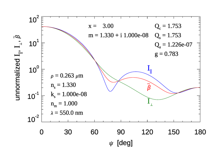
As a first example, let us reproduce one of the figures from Bohren and Huffman (1983). They considered a water droplet in air with $\rho =0.263\mu m$, an index of refraction of the particle relative to the air of $m=1.33+i10^{-8}$, and a wavelength of $\lambda =550nm$. These values give a size parameter of $x=3$. Figure 1 shows the curves for $I_{\perp }=|S_1{|}^2$, $I_{\parallel }=|S_2{|}^2$, and $\tilde{\beta }=\frac{1}{2}\left(I_{\perp }+I_{\parallel }\right)$. The $I_{\perp }$ and $I_{\parallel }$ curves exactly reproduce the curves in Fig. 4.9(b) of Bohren and Huffman. This is a check that the Mie code is working correctly.

The $I_{\perp }$ and $I_{\parallel }$ curves can be viewed as unnormalized phase functions for scattering of incident light that is polarized perpendicular (parallel) to the scattering plane into light that is polarized perpendicular (parallel) to the scattering plane. The red curve shows the phase function for scattering of unpolarized incident light into a sensor that is not polarization sensitive. This is the phase function usually used by oceanographers. Recall, however, the warning of the previous page about Mie codes outputting unnormalized amplitude matrix elements. Integrating the red curve of Fig 1 gives

Thus the red curve in the figure must be divided by 51.37 to obtain a properly normalized phase function that could be used, for example, in HydroLight.

The figure also shows the scattering, absorption, and attenuation efficiencies, and the mean cosine of the scattering angle. The scattering efficiency $Q_s$ is 1.753, which means that the particle is scattering more than would be expected from its geometric cross section $\pi {\rho }^2$. We will return to this peculiar result below.

Example 2: Oceanic Particles

Let us next consider a particle that might be an approximation to a small spherical phytoplankton like Synechococcus. For physical parameters we use

• $\rho =0.5\mu m$
• $n_s=1.37$
• $k_s=0.015$ (corresponding to $a_s=3.77\times 10^5{m}^{-1}$)
• $n_m=1.33$
• $\lambda =500nm$

(Remember that the absorption coefficient $a_s$ is the absorption coefficient of the plankton material. These values are typically in the range of $10^4$-$10^5{m}^{-1}$ at visible wavelengths.) Figure 2 shows the resulting normalized phase function for unpolarized light.

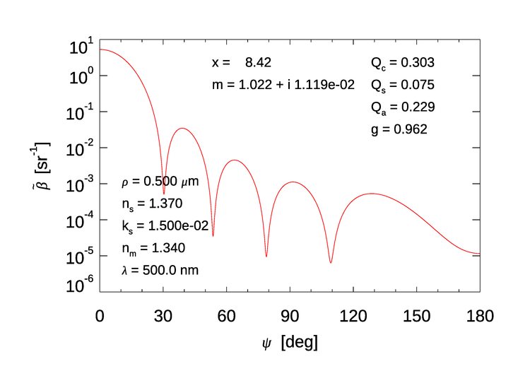
As seen in this figure, a single particle scatters light in a very complex angular pattern. The peaks and valleys of the phase function result from constructive and destructive interference between the incident electric field and the field that arises in the region of the sphere. You can think of this as being the 3D version of the diffraction pattern of bright and dark lines seen when a plane wave is incident onto a slit in screen (see, for example, Fig. 1 on the Nature of Light page). You can also think of this pattern as resulting from the sum of the infinite series of multipole modes of the scattered field, that is, the sum of a dipole electric field, plus a quadrapole field, plus an octopole field, plus....

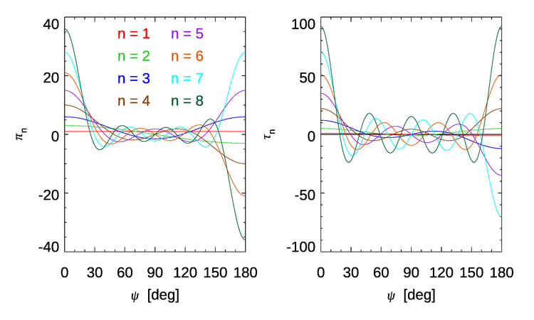
Recall from Eq. (6) of the Mie Theory Overview page that the amplitude matrix elements are given by infinite sums of particle-dependent coefficients (the $a_n$ and $b_n$ of Eq. (7)) times angle-dependent functions ${\pi }_n\left(\psi \right)$ and ${\tau }_n\left(\psi \right)$ given by Eq. (8) of that page. Figure 3 shows the first 8 of the angle functions. The most important feature to note in these curves is that both ${\pi }_n$ and ${\tau }_n$ are always positive as $\psi \to 0$. Therefore, as more and more terms are added in the amplitude matrix sums, the small-angle amplitudes (hence the associated phase function) become more and more peaked. The oscillations at larger scattering angles combine to create the peaks and valleys of seen in the phase functions of Figs. 1 and 2 and in 5 below.

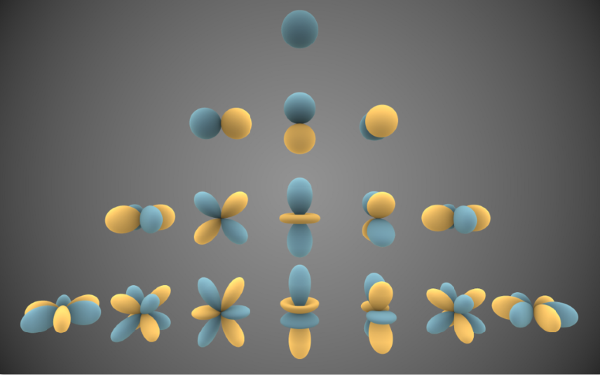
The shapes of the ${\pi }_n$ and ${\tau }_n$ functions trace back to mathematical functions called spherical harmonics, which are buried deep inside the Mie equations. Expanding a 3D function of $\left(𝜃,\varphi \right)$ as a sum of spherical harmonics is analogous to expanding a 1D function as a sum of sines and cosines (a Fourier series). Figure 4 shows a graphical representation of the first few spherical harmonics. (If you think these patterns looks suspiciously like the shapes of the orbitals seen in Fig. 1 of the Physics of Absorption, you would not be wrong. The underlying physics is different—quantum mechanics vs light scattering—but the same mathematical functions crop up on both cases.)

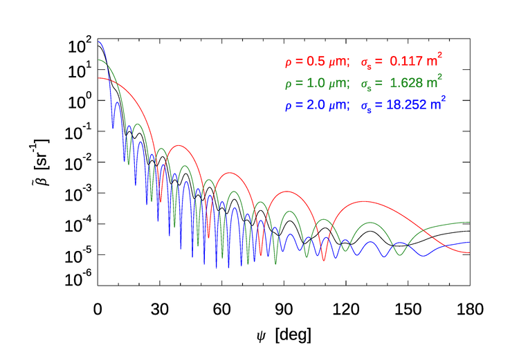
The locations of the peaks and valleys of the scattering pattern depend on the particle’s physical properties—its size, relative index of refraction, and the wavelength. Figure 5 shows three normalized phase functions for the same particle type (a simulated phytoplankton) as in Fig. 2, but for particles of radii $\rho =0.5,1.0,2.0mum$. These particles have size parameters of $x=8.42,16.84$, and 33.68, respectively; each particle has $m=1.02239+i0.01119$. It is seen that the peaks and valleys of the phase functions are at different scattering angles. In general, the larger the size parameter $x$, the more features there are in the phase function. Note also that as the particle size increases, the phase function becomes more peaked at small scattering angles. The scattering cross section increases rapidly with particle size; that is, a large particle scatters more strongly than a small particle.

In the ocean, there are particles of many sizes and many indices of refraction, all occurring with different numbers of particles per cubic meter. When the phase functions for many different particle sizes and compositions are added together, the peaks and valleys of the individual phase functions tend to cancel out, leaving a much smoother phase function for the mixture of particles corresponding to what is measured on a sample of ocean water.

To combine phase functions for different particle types or sizes, remember that IOPs, including the volume scattering function, are additive. Thus the total phase function for the three particles used to generate Fig. 5 would be combined as follows. Let ${\mathcal{𝒩}}_i,i=1,2,3$ be the number density (particles per cubic meter) of each size of particle. The particle scattering cross sections obtained from Mie theory are ${\sigma }_{si}$; the values are shown in Fig. 5. Then

Suppose, just for the sake of illustration, that there are one-fifth as many particles of radius $\rho =1\mu m$ as there are particles of radius $\rho =0.5\mu m$, and one-fifth as many of radius 2 as of radius 1. Then the three individual-particle phase functions seen in the red, green, and blue curves of Fig. 5 would combine to give the total phase function shown by the black curve in the figure. This shows that the highly peaked features of the single-particle phase functions are starting to average out to leave a smoother total phase function. When the same process is carried out for many sizes of particles, say from 0.1 to $100\mu m$, and for many different kinds of particles (living phytoplankton of various types, detritus, sediment particles, etc.), a much smoother, typical ocean phase function can result.

Adding the results for individual particles together in the manner just shown assumes that each scattering particle is in the “far field” of its neighbors, so that the scattered field set up by one particle is not affected by nearby particles. This means that the particles should be separated by many wavelengths of the light. If there are, say, $10^{12}$ particles per cubic meter (a typical value for small phytoplankton) and the wavelength is 500 nm, then each particles is separated by 200 wavelengths, on average. This more than satisfied the far-field approximation.

Note, however, that the relative contributions of different particles is highly dependent not just on particle size and index of refraction, but on how many particles there are. Very small particles generally occur in high numbers, but they are individually weak scatterers and thus may contribute little to the total because of their small cross sections. Very large particles are strong scatterers, but they occur in very small numbers, and thus also may contribute little because of their small numbers. It is often the medium-sized particles, say radii from 0.5 to $5\mu m$, that contribute the bulk of the total scattering in typical waters.

The Extinction Paradox

Recall from Fig. 1 that the scattering efficiency was $Q_s=1.753$ for a small water droplet in air at 550 nm. This says that the particle is scattering more light than just the light that encounters the cross-sectional area of the particle. This seems counterintuitive from everyday experience. If light hits a baseball, some will be absorbed and some will be reflected (scattered) by the ball, but light that misses the ball travels onward—or so it seems.

Figure 6 shows the absorption ($Q_a$), scattering ($Q_b$), and extinction ($Q_c=Q_a+Q_b$) efficiencies for highly absorbing soot particles, which are generated by incomplete combustion and are a common component of air pollution caused by coal-fired power plants, diesel exhaust, or forest fires. Soot has a real index of refraction of about 1.5, and an imaginary index of about 0.05 (Adler et al. (2010)). The wavelength of the incident light is 532 nm.

For small size parameters, starting from $x=0$, the scattering curve rises rapidly and then displays broad but damped oscillations with increasing $x$. These oscillations are caused by constructive and destructive interference between the incident and scattered light waves. Thus very small particles can be very efficient scatterers if their size matches the wavelength of the light in just the right way. For these soot particles in air, the maximum in scattering efficiency near $x=4$ corresponds to a particle radius of about 340 nm. There is also a fine “ripple structure,” which requires a more complicated explanation (see Bohren and Huffman (1983)). Thus these very small particles are scattering much more energy than would be expected from their physical cross section size. This behavior of large extinction for small $x$ is seen in measurements of soot extinction efficiency in Fig. 7. The agreement between measurements and Mie theory is surprisingly good given that real soot particles are far from spherical.

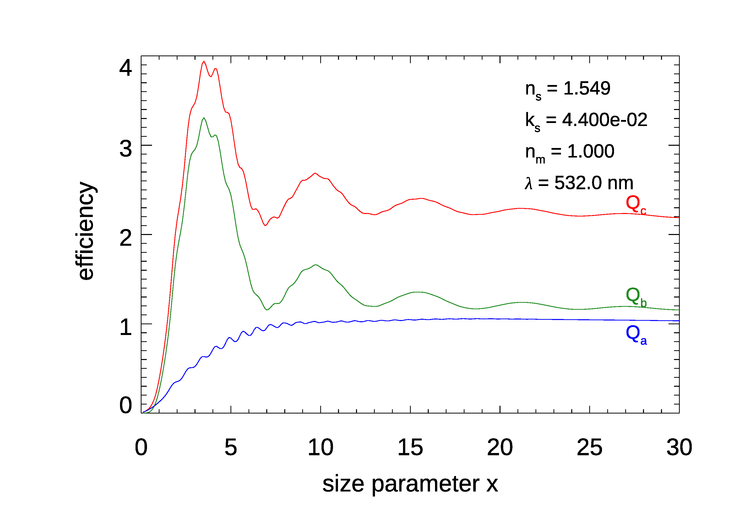
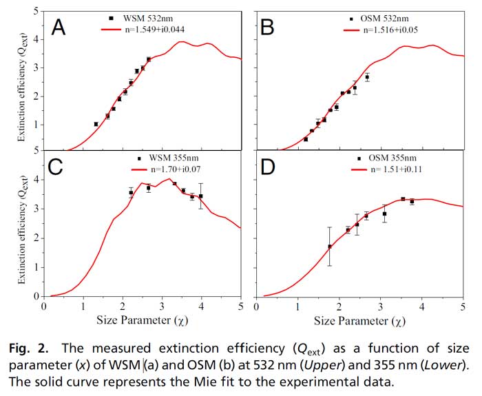
Figure 6 shows that, for soot in air, as $x$ becomes large, $Q_a$ is close to 1, but so is $Q_b$, so $Q_c$ is close to 2. These values remain similar as $x$ continues to increase. For $x=10,000$ (a particle size of $\rho =0.85mm$ for $\lambda =532nm$), $Q_a=0.9085$, $Q_b=1.096$, and $Q_c=2.004$. The $Q_a$ value makes sense: the soot is highly, but not totally absorbing, so a 91% absorption efficiency is plausible. However, if the light incident onto the particle is almost all absorbed, then it would seem that the particle should not be scattering as much or more light as it absorbs.

Geometric optics is a model of light propagation using rays and is often used to model light scattering by objects that are much, much larger than the wavelength of light. Geometric optics corresponds to large size parameters $x$ in Mie theory. Geometric optics predicts that the maximum of $Q_c$ should be 1, that is, a particle can absorb and/or scatter at most the energy that is incident onto the particle. The asymptotic approach of $Q_c$ to 2 is known as the “extinction paradox.” This very general result is called a paradox because geometric optics predicts $Q_c=1$. An equivalent statement is that the asymptotic value of the extinction cross section ${\sigma }_c$ is twice the particle’s geometric cross section $\pi {\rho }^2$.

The standard explanation for the extinction paradox is that the “extra” scattering is due to diffraction by the particle. The electric field of light passing near to, but not intersecting, the particle is perturbed by the presence of the particle, which causes the light to change direction. Diffraction is not easily observed for everyday objects like baseballs because the angle of deviation of the diffracted light from the direction of the incident light is extremely small. Indeed, it was Newton’s inability to observe the bending of light around large objects, and their apparently sharp shadow edges, that led him to conclude that light consisted of particles and not waves. Nevertheless, diffraction occurs for all sizes of objects, and any deviation, no matter how small, of light from its initial direction counts as scattering and contributes to $Q_b$. However, the diffraction explanation can be shown to be incomplete, and papers are still being written about the fundamental cause of the $Q_c=2$ limit (e.g., Berg et al. (2011)). The full explanation requires a deep understanding of how the incident and scattered waves interact within and surrounding the particle. Regardless of the full explanation, the effect is very real and occurs for all particles.

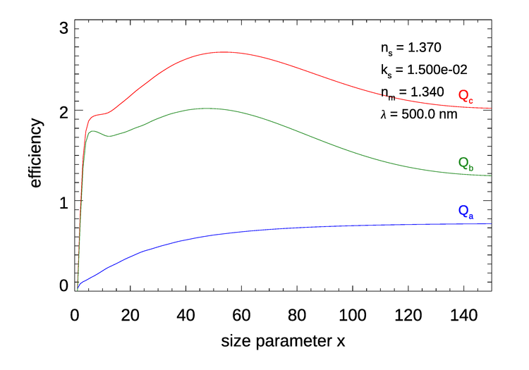
Another example of the extinction paradox is seen in Fig. 8. These simulations are for quartz particles in water. Quartz has a real index of refraction of about 1.54 and is modeled here as completely non-absorbing. The wavelength is taken to be 500 nm. Since the particles are non-absorbing, the absorption efficiency is identically 0, and the total extinction is due to scattering ($Q_c=Q_b$). Both the interference structure and the ripple structure are clearly seen. The ripple structure is much less noticeable for the soot particles in Fig. 6 because the ripples are damped out by absorption. The quartz particles also display an oscillating, asymptotic approach of $Q_c$ to a value of 2, just as do the soot particles.

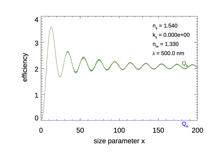
Figure 9 shows the efficiencies for the phytoplankton model used to generate the phase function of Fig. 2. For this relative index of refraction, the scattering efficiency shows only one broad maximum near $x=50$, which corresponds to a particle radius of about $\rho =3\mu m$. By $x=150$, the extinction efficiency $Q_c=2.02$, so within 1% of its asymptotic value.

A fine way to spend a rainy Saturday is to download a Mie code and do a few thousand runs to see the effects of real and imaginary indices of refraction, particle size, and wavelength on the various phase functions and efficiencies. However, regarding the wavelength effect, keep in mind that as wavelength changes so do the indices of refraction of the particle and medium. Suppose that, for a given particle radius $\rho$ you want to generate a figure like Figs. 9 and 8, but showing the efficiencies as a function of wavelength. That can be done, but you have to change the particle and medium indices of refraction for each wavelength. The absorption coefficient of water changes from $a_w\approx 0.015m^{-1}$ at 440 nm to $0.65m^{-1}$ at 700 nm. If modeling a water droplet in air, this wavelength dependence of $a_w$ determines the water imaginary index of refraction via $k_s\left(\lambda \right)=a_w\left(\lambda \right)\lambda ∕\left(4\pi \right)$, and thus affects the size parameter $x\left(\lambda \right)=2\pi \rho k_s\left(\lambda \right)n_m\left(\lambda \right)∕\lambda =\rho a_w\left(\lambda \right)n_m\left(\lambda \right)∕2$. If modeling a phytoplankton in water, the needed phytoplankton $k_s\left(\lambda \right)$ might be constructed from a phytoplankton chlorophyll-specific absorption spectrum, and so on.

Finally, remember that Mie theory is valid only for homogeneous spherical particles, even though it often, but not always, gives reasonable approximate results for non-spherical particles.