Page updated:
March 13, 2021
Author: Curtis Mobley
View PDF
Raman Scattering
First of all, the pronunciation is RAman, not raMAN. Raman scattering is a type of inelastic scattering of light by molecules. Compton scattering (see The Nature of Light) is inelastic scattering of X-rays by electrons. Upon learning of Compton’s discovery (for which Compton received the 1928 Nobel Prize in Physics), C. V. Raman thought there should be a similar effect at visible wavelengths and set out to find it. He succeeded and subsequently received the 1930 Nobel Prize for the discovery and explanation of what is now called Raman scattering or the Raman effect. (Incidentally, Raman received his bachelor’s degree in physics at 16, graduating at the head of his class, and he published his first paper at 18. The Raman family produced a number of scientists, included Raman’s nephew Subrahmanyan Chandrasekhar, who received the Nobel in 1983. The family seems to have had good genes for science.)
The physics of Raman scattering is quite complicated, but it can be conceptualized as following. Incident light can excite a molecule in its ground state to a higher “virtual” energy level, which then immediately decays back to a lower level accompanied by the emission of light. If the decay returns the molecule to its initial state, the scattering is elastic and is called Rayleigh scattering. If the decay is to a molecular vibrational level above the ground state, then then emitted light has a longer wavelength (lower energy) than the incident light: this is Raman scattering. (See The Physics of Absorption for a discussion of electronic, vibrational, and rotational energy levels.) The use of Raman scattering, often called Raman spectroscopy, is widely used in chemistry as a way to study the vibrational energy levels of molecules. In those applications, the incident light usually comes from a laser. In the ocean, the molecule of interest is water, and the exciting light can be either sunlight or a laser.
The wavelength shift for Raman scatter by water is exceptionally large, corresponding to a wavenumber (1/wavelength) shift of about , which at visible wavelengths is many tens to more than a hundred nanometers. The time scale for Raman scattering (i.e, the time for the molecular excitation and subsequent decay) is roughly to seconds. This is much faster than the time scale of fluorescence by chlorophyll or CDOM molecules, which is on the order of or longer. Thus Raman scatter can be thought of as an almost instantaneous scattering process, rather than as the absorption of light followed much later by the emission of new light.
Quantities Defining Raman Scattering
The quantities needed to compute Raman scatter contributions to the radiance are
- the Raman scattering coefficient , with units of
- the Raman wavelength distribution function , with units of
- the Raman scattering phase function beta , with units of
The next sections discuss each of these quantities in turn.
The Raman scattering coefficient
The Raman scattering coefficient tells how much of the irradiance at the excitation wavelength scatters into all emission wavelengths , per unit of distance traveled by the excitation irradiance. The most recently published values of for water are (Bartlett et al. (1998)) and (Desiderio (2000)). (The current version (6.0) of the HydroLight radiative transfer model uses as the default value.)
Various values for the wavelength dependence of can be found in the literature. Bartlett et al. (1998) reviewed the wavelength dependence of the Raman scattering coefficient in detail and found, based on their measurements, a wavelength dependence of for calculations performed in energy units (as in HydroLight). In terms of the excitation wavelength, Bartlett et al. found for energy computations. (The current version of HydroLight uses as the default.) For calculations in terms of photon numbers (as in a Monte Carlo simulation), Bartlett et al. found wavelength dependencies of or .
The Raman wavelength distribution function
The Raman wavelength distribution function relates the excitation and emission wavelengths, i.e., what wavelengths receive the scattered spectral irradiance for a given excitation wavelength or, conversely, what wavelengths excite a given emission wavelength . (The term “wavelength distribution function” is non-standard, but descriptive, so that is what was used in Light and Water and again here.) The function is most conveniently described in terms of the corresponding wavenumber distribution function , where is the wavenumber shift, expressed in units of . This follows because the Raman-scattered light undergoes a frequency shift that is determined by the type of molecule and is independent of the incident frequency. The wavenumber in is related to the wavelength in nm by , and to the frequency by , where is the speed of light. (The factor converts nanometers to centimeters.)
According to Walrafen (1967), the shape of for water is given by a sum of four Gaussian functions:
| (1) |
where
- is the wavenumber shift of the Raman-scattered light, relative to the wavenumber of the incident light, in
- is the center of the Gaussian function, in
- is the full width at half maximum of the Gaussian function, in
- is the nondimensional weight of the Gaussian function.
The values of , , and for pure water at a temperature of 25 deg C are given in Table 1. Figure 1 shows evaluated for the water parameter values of Table 1. The function shows a peak and a shoulder, which result from the sums of the four gaussians seen in Eq. (1). For water, the wavenumber shift is roughly .
| | |
||
| 1 | 0.41 | 3250 | 210 |
| 2 | 0.39 | 3425 | 175 |
| 3 | 0.10 | 3530 | 140 |
| 4 | 0.10 | 3625 | 140 |
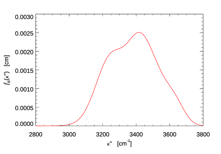
Consider, for example, incident light with , which corresponds to . Figure 1 shows that this light, if Raman scattered, will be shifted by roughly to , which corresponds to .
The function can be interpreted as a probability density function giving the probability that a light of any incident wavenumber , if Raman scattered, will be scattered to a wavenumber
| (2) |
The function satisfies the normalization condition
| (3) |
as is required of any probability distribution function. The integration limits above come from observing that as then the wavenumber , and as then . If A change of variables from to in Eq. (3) leads to the corresponding wavelength redistribution function . Thus
where the wavelengths are in nanometers. In the last equation, we have identified the function
| (4) |
as being the desired Raman wavelength redistribution function, with units of .
In we can fix the incident wavelength and plot the corresponding emission wavelengths. We can also fix the emission wavelength and use the function to see where the light emitted at comes from. Both options are seen in Fig. 2.
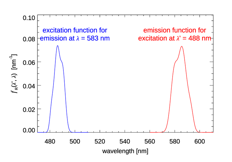
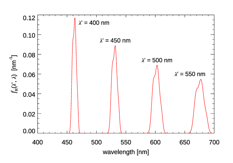
Figure 3 shows for four values of the incident wavelength . These plots show that as the incident wavelength increases, the emission band becomes broader and the shift from to becomes larger. Excitation at 400 nm gives emission centered at roughly 463 nm, a shift of 63 nm, but excitation at 550 nm gives emission centered at round 677 nm, a shift of 127 nm.
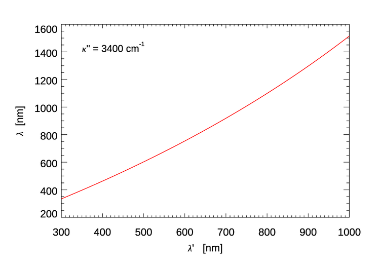
Equation (2) can be rewritten as
and used to compute the approximate center of the emission wavelength band for a given excitation wavelength. Figure 4 shows the result.
The Raman phase function
The Raman phase function gives the angular distribution of the Raman scattered radiance. This function (averaging over all polarization states) is given by
where is the scattering angle between the direction of the incident and scattered radiance, and is the depolarization factor. The value of depends on the wavenumber shift (Ge et al. (1993), their Fig. 2). For a value of , , in which case the phase function is
This phase function is similar in shape to the phase function for elastic scattering by pure water.
Incorporation of Raman Scatter into Radiative Transfer Calculations
We now have have the pieces needed to define the volume scattering function for Raman scattering, , where and represent the incident and final directions of the light. This VSF specifies the strength of the Raman scattering via the Raman scattering coefficient , the wavelength distribution of the scattered light via the wavelength redistribution function , and its angular distribution relative to the direction of the incident light via the Raman phase function . Thus we have
| (5) |
Raman scatter is incorporated into unpolarized radiative transfer calculations as a source term (See Eq. 3 of The Scalar Radiative Transfer Equation):
The scattering angle is given by , which can be computed from via Eq. (5) of the Geometry page.
Note that this formidiable equation cannot be solved at just the wavelength of interest; it must be solved at all wavelengths that contribute Raman-scattered radiance to the radiance at .
Examples of Raman Effects
Effect on remote-sensing reflectance
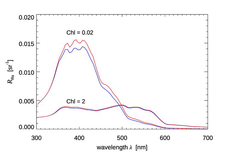
Figure 5 shows the effect of Raman scattered radiance on the remote-sensing reflectance for chlorophyll values of and as simulated by HydroLight. The HydroLight runs used a bio-optical model for Case 1 water for which the absorption and scattering properties of the water are determined only by the chlorophyll concentration. The water was homogeneous and infinitely deep. The Sun was at a 30 deg zenith angle in a clear sky; the wind speed was . Identical runs were made with and without Raman scatter included in the runs. It is seen that for the very clear water with , is as much as 22% higher, but for the water with , Raman increases by at most 5%. The Raman effect decreases but still can be significant in higher chlorophyll waters or in turbid Case 2 waters. Although difficult to see in Fig. 5, the Raman effect does not “turn on” until about 340 nm even though the HydroLight run started at 300 nm. This is because the start of the emission band for excitation near 300 nm is around 340 nm (recall Fig. 4).
Effect on upwelling plane irradiance
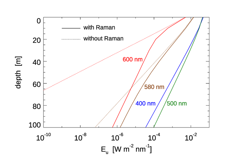
Although Raman scattering does not have a large effect on except in the clearest water, it can be the dominant source of light at red wavelengths at depths where absorption by water has removed most of the incoming sunlight. This is illustrated in Fig. 6. HydroLight was run for Case 1 water with a chlorophyll concentration of , which is typical of open ocean water. The Sun was at a 30 deg zenith angle in a clear sky. The run started at 300 nm, so that Raman effects would be present at wavelengths greater than 340 nm. At 400 and 500 nm, the contribution by Raman scattered light to the upwelling irradiance is almost unnoticeable. This is because at these wavelengths elastically scattered solar radiance is the main contributor to the upwelling irradiance. At 580 nm, water absorption () is beginning to filter out enough of the solar radiance that the Raman contribution, which comes from wavelengths around 485 nm (see Fig.4), where the light penetrates well to depth, is becoming the main contribution to . At 600 nm, water absorption () has removed almost all of the solar light below about 20 m. Below 20 m, almost all of comes from Raman scattered light that originates from wavelengths around 500 nm, where sunlight penetrates well to depth. It should be noted that below about 40 m, the depth rate of decay of (i.e., ) is almost the same as the rate of decay the irradiance at 500 nm. This is because the light at 500 nm is the source of the light at 600 nm.
It was the measurement of unexpected upwelling irradiance at depths below 50 m and wavelengths greater than 520 nm that led Sugihara et al. (1984) to suggest that the unexpected upwelling irradiance came from downwelling irradiance a blue-green wavelengths being Raman scattered. A number of subsequent studies (e.g., Stavin and Weidemann (1988), Marshall and Smith (1990)) confirmed this hypothesis. Many studies since have studied Raman effects on ocean light fields. For example, Kattawar and Xu (1992) and Ge et al. (1993) studied the filling in of Fraunhofer lines in underwater light by Raman scattering.
Interpretation of Raman emission profiles
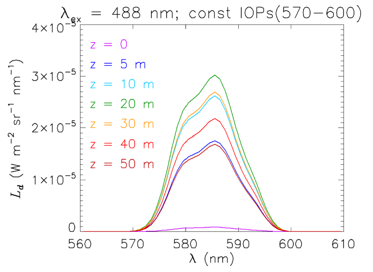
Another interesting example of the contribution of Raman scattering to in-water radiances is seen in Fig. 7. This plot shows the downwelling (zenith-viewing) radiance generated from a HydroLight run using its option for simulating LIDAR illumination at one wavelength in an otherwise black sky. The inputs were as follows:
- The incident (LIDAR) irradiance was at 488 nm; the sky was otherwise black.
- The chlorophyll concentration was for Case 1 water
- The water was infinitely deep water with Eq. (6) solved down to 50 m
- The output was at 560 to 610 nm at 1 nm resolution

The curves in Fig. 7 are explained as follows. At depth 0, just below the sea surface, the only contribution to is upwelling radiance that is reflected back downward by the sea surface. By 5 m depth, there is now enough water above the simulated measurement instrument that the water column is generating significant downwelling radiance. Note that the shape of the emission has the same shape as the emission function seen in Fig. 2, namely a peak near 585 nm with a shoulder at about 580 nm. As the depth increases to 10 and then 20 m, the magnitude of increases, but the shape of the emission begins to flatten between 580 and 585. By 30 m, the magnitude of has decreased because of the decrease in the radiance penetrating to this depth from the water between the surface and 30 m, and the magnitude continues to decrease as the depth becomes greater. However, the shape of the emission at 30 m shows almost the same magnitudes at 580 and 585 nm, and at 40 and 50 m, the peak emission is actually greater at 580 than at 585 nm. This may seem strange because the shape of the Raman emission function seen in Fig. 2 is the same for all depths.
This “reversal” of the “peak-shoulder” shape of the emission is a consequence of the difference in absorption across the emission wavelengths. The total absorption (water plus phytoplankton) increases by a factor of three (from 0.071 to ) between 570 and 600 nm, and by 22% (from 0.091 to ) between 580 and 585 nm. These rapidly increasing absorption values change the shape of the local (at each depth) emission function when integrated over depth to obtain the total , which has contributions from all depths. Simply stated, the higher absorption at the 585 nm peak lets relatively less of the radiance emitted above a given depth reach the measurement depth than for the shoulder at 580 nm, so the 585 nm peak appears smaller relative to the shoulder than what is seen for the emission function of Fig. 2.
The claim that the change is shape with depth of the Raman emission is due to wavelength-dependent absorption can be verified as follows. An “artificial water” IOP data file was created with the IOP values between 570 and 600 nm having the values at 570 nm. The water IOPs are then the same over the entire range of emission wavelengths seen in Fig. 7. The resulting Raman spectra are seen in Fig. 8. Now, without the wavelength-dependent absorption, the shape of does not change with depth and, indeed, looks exactly like the shape of the emission function seen in Fig. 2. The magnitude of the curves is greater than before because the absorption is less. Of course, if the HydroLight run had been made at 5 or 10 nm resolution, then the shape of the emission band would not have been resolved. However, the total Raman-scattered power would have been the same, but spread over the wider bands.
These simulations show that the interpretation of Raman-scattered spectra can be complicated because of IOP effects at both the excitation and emission wavelengths, even in the simplest possible case of excitation at one wavelength in an otherwise black sky. The situation becomes even more complicated for solar-stimulated Raman scatter because many excitation wavelengths can contribute to a range of emission wavelengths, and everything blurs together in a non-obvious fashion.
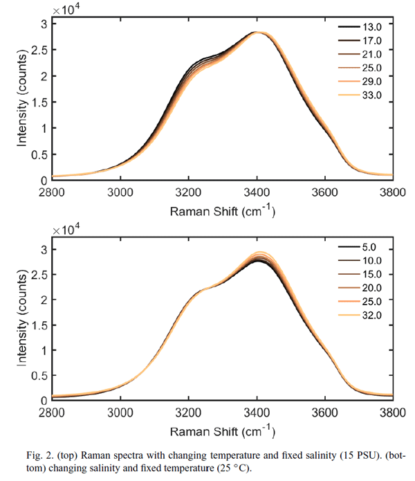
Temperature and Salinity Dependence
The Walrafen data presented in Table 1 were determined on pure water at a temperature of 25 deg C. There is, however, a small but significant dependence on temperature and salinity of the shape of the emission curve seen in Fig. 1. This dependence is shown in Fig. 9. The upper panel shows the shape of the emission curve as a function of temperature for a salinity of 15 PSU, and the lower curve shows the dependence on salinity for a temperature of 25 deg C. Artlett and Pask (2017) have shown in laboratory measurements that these differences can be used to simultaneously determine temperature and salinity with an RMS errors of and , and they present the design for a three-channel Raman spectrometer that excites at 532 nm and measures the emission at three bands. The emission bands would be used to form band ratios, from which temperature and salinity can be extracted.
 See comments posted for this page and leave your own.