Page updated:
May 19, 2021
Author: Curtis Mobley
View PDF
Beam and Point Spread Functions
This page defines two equivalent quantities that describe light propagation in absorbing and scattering media and that are fundamental to image analysis.
The Beam Spread Function
Consider a collimated source emitting spectral power (units of ) in direction as shown in Fig. 1. As the beam passes through the medium, scattering will spread out the beam as illustrated by the green arrows in the figure, and absorption will reduce the beam power. The combined effects of scattering and absorption give some spectral plane irradiance (units of ) on the surface of a sphere of radius at an off-axis angle relative to the direction of the emitted beam. The irradiance sensor used to measure has a cosine response for angles relative to the normal to the detector surface. It is assumed here that the emitted light is unpolarized and that the medium is isotropic, so that there is no azimuthal dependence of the detected irradiance. The green arrows in the figure represent one possible path for light between the source and the detector.
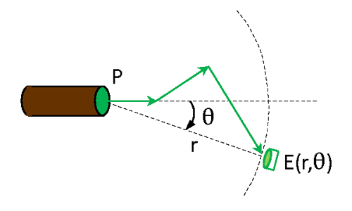
The beam spread function (BSF) is then defined as the detected irradiance normalized by the emitted power:
| (1) |
Recall that the Volume Scattering Function (VSF) describes a single scattering event. Two such scatterings are shown for the green arrows in Fig. 1. The BSF on the other hand describes the cumulative effects on the emitted beam of all of the scattering and absorption events between the source and the detector. The BSF thus depends on the distance between the source and the detector, whereas the VSF depends only on the optical properties of the medium and is independent of the locations of the source and detector.
The Point Spread Function
Now suppose that there is a source at the location of the detector in Fig. 1 and that this source is emitting spectral intensity (units of ) with an angular pattern given by
For this intensity pattern the total emitted power is
The short green arrows in Fig. 2 illustrate the emission of light by this cosine source. As illustrated by the long green arrows in this figure, the emitted intensity will give rise to a radiance , where is the distance from the source and is direction measured from the axis of the emitted intensity. The light emitted by this source is then detected by a well collimated radiance sensor that can scan past the source as shown in Fig. 2.
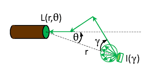
The Point Spread Function (PSF) is then defined as the detected radiance normalized by the maximum of the emitted intensity:
The PSF can be visualized as the “glow” of light around distant street light seen through a foggy atmosphere as seen in Fig. 3. Although a street light is not a cosine-emitting point source, the angular pattern of the glow seen around the light gives a qualitative feeling for the PSF, which is just the pattern of the radiance distribution centered on the source.
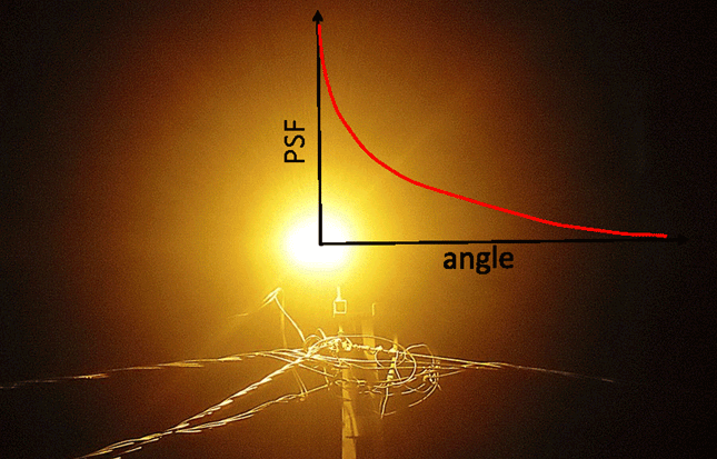
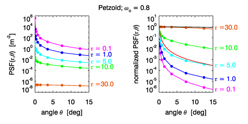
Figure 4 shows PSFs computed by Monte Carlo simulations for a homogeneous water body with a Petzold average particle phase function and a single-scattering albedo of . The left panel shows the PSF for the first 15 deg of and for nondimensional optical distances between the source and detector of = 0.1, 1, 5, 10, and 30. These curves show that the magnitude of the PSF decreases as increases because of absorption. The colored dots are the centers of the angular bins used to tally the light rays in the Monte Carlo simulations.
The right panel of the figure shows the PSF values normalized to 1 at . These curves show that the shape of the PSF starts out very highly peaked near for small and eventually becomes relatively flat in as the optical distance increases. This is progression of PSF shapes can be understood as follows.
As goes to zero, there is almost no chance for light to scatter. As the radiometer seen in Fig. 2 scans past the point source, it sees either almost nothing, or it sees the point source at . The PSF then approaches a Dirac delta function in as . As the optical distance increases, there is more and more chance for scattering until many photons have been scattered once. The PSF then begins to look similar to the scattering phase function, which describes the redistribution of radiance by single scattering. The red curve lying close to the curve for is the normalized Petzold phase function used in these simulations. (The PSF would not in general ever have exactly the same shape as the phase function. Even if, at some distance, most light rays have been scattered once, others will not yet be scattered, and others will have been scattered more than once. Thus a PSF never describes just single scattering.)
Finally, as becomes very large, all rays have been scattered many times, and the resulting radiance distribution, hence the PSF, approaches the shape of the asymptotic radiance distribution . The black curve near the PSF shows as computed by HydroLight for the IOPs of these simulations. The curve is still noticeably different from . It is computationally expensive to trace enough rays to large optical distances to reproduce the asymptotic distribution. A computation for required emitting initial rays, of which about 0.05% reached for deg, but the resulting PSF (not shown) is much closer to . Similarly, statistical noise can become large for large angles if the angular bins are small. However, it is the small values that are most important for image analysis (after all, you are usually looking generally toward an object, not away from it), so noise at large angles is seldom a problem in practical applications.
Equivalence of the BSF and PSF
In Maxwell’s Equations for the propagation of electromagnetic energy, if you change time to minus time, nothing changes except that the direction of propagation is reversed. This means that if light is propagating from the source to the receiver along the path shown in Fig. 1, then light emitted from the receiver location in the same direction as the detected beam will propagate back along the same path to the source, as shown by the green arrows in Fig. 2. This is known as the principle of electromagnetic reciprocity, or Helmholtz reciprocity, or the “if I can see you, you can see me” theorem. Figures 1 and 2 were drawn to highlight the symmetry between the BSF and the PSF.
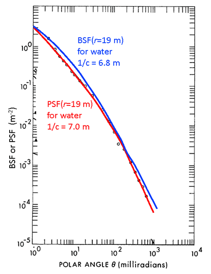
The BSF and PSF are superficially different: a collimated source and a cosine detector vs a cosine source and a collimated detector. However, reciprocity suggests that the BSF and PSF contain equivalent information. Indeed, the BSF and PSF are numerically the same. Figure 5 shows PSF and BSF measurements from two very similar water bodies obtained by Mertens and Replogle (1977). The instruments were mounted on a 20 m long underwater frame, which allowed a maximum range between source and detector of approximately 19 m. Although the measurements in the figure were made on different days and the water IOPs were slightly different, the closeness of the PSF and BSF over several orders of magnitude suggests that the BSF and PSF are numerically equal, as they stated without proof. Gordon (1994b) started with the radiative transfer equation and used reciprocity to show that the BSF and PSF are indeed numerically equal. It is thus customary refer to just the PSF, even if the geometry of a problem corresponds to that of the BSF. (This is the case in the derivation of the Lidar equation, for example.)
Importance of the PSF in Image Analysis
The PSF plays a fundamental role in the prediction of how an object appears when seen through an absorbing and scattering medium such as water. Suppose you are looking in a particular direction at point in Fig. 6 from a distance away from the shark. Most of the light detected in this viewing direction probably comes from point in the image. However, every other point in the scene contributes at least a small amount of light to the detected signal in the viewing direction because of scattering from those other directions into the viewing direction. How much light those other points contribute to a given direction is determined by the value of their PSFs at the angular distances away from the viewing direction.
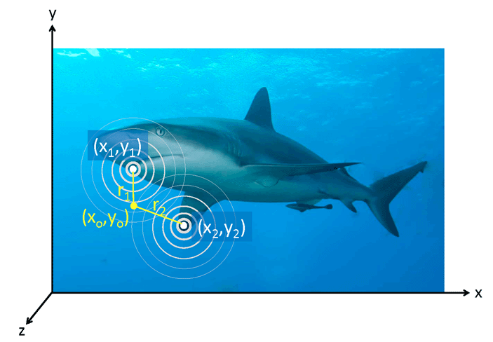
Let represent the “bright-dark” pattern of the shark image when seen at distance , or as seen through a vacuum. Thus for a gray-scale digital image and 8 bit resolution, for a black pixel and for white pixel. When viewing a particular point in the image through a vacuum at some distance from the shark, the detected radiance comes only from point and has the value . However, when viewing point in the through a scattering medium, every point in the scene contributes to the radiance seen at . The concentric white circles in the figure represent contours of . Point thus contributes a radiance of , where angle . Likewise point contributes radiance , where angle . The total radiance at point is given by summing up the contributions from all points in the image:
| (2) |
The connection between points in the image at distance away and the distance and angular variables used for PSFs is
so that
Thus, given the inherent appearance of an object (the appearance at distance or through a vacuum) and the PSF of the medium, the appearance of the object as seen through the medium can be computed. In other words, the PSF completely characterizes the effect of the environment on an image.
Note that in a vacuum and with a perfect optical system, the PSF reduces to a 2D Dirac delta function: , in which case
Thus the image at distance is the same as at distance 0.
Integrals of the form
| (3) |
are called convolution integrals, and is called the convolution of and . Equation (2) is a two-dimensional convolution showing that the image seen from a distance is the convolution of the image seen from zero distance and the PSF of the medium at distance . This is an extremely important result and is the foundation of image analysis through absorbing and scattering media. As will be seen in the Photometry and Visibility Chapter (under development), the Fourier transform of Eq. (2) has very useful properties. Rather than compute the double integral of Eq. (2) for every point of the scene (which is computationally inefficient), the Fourier transforms of and can be computed (computationally efficient using Fast Fourier Transforms), multiplied, and then the inverse transform of the product gives the final image. This topic will be developed in the Level 2 pages of the Photometry and Visibility chapter. Meanwhile see Mobley (2020), Goodman (1996), or the Mertens and Replogle paper cited above. Hou et al. (2007) used this equation as the starting point for a rigorous analysis of the visibility of a Secchi disk.
Because of the importance of the PSF in image analysis, considerable effort has been expended to develop models of the PSF as a function of water IOPs. A number of such models are reviewed in Hou et al. (2008). The page on The Lidar Equation shows the fundamental role of the BSF in lidar remote sensing.
Comment on terminology
he term “convolution” is frequently misused. An integral of the form is not a convolution. It can be called the inner product of and , or the integral of weighted by (or of weighted by ), but it returns a number. The convolution of and returns a functional as shown in Eq. (3). At best, you could call the value of the convolution at , but that is missing the central idea that a convolution shows how two functions “overlap” so that, in the case of an image, each point in an image contributes to all other points.]
 See comments posted for this page and leave your own.