Page updated:
February 10, 2021
Author: Curtis Mobley
View PDF
Thematic Mapping
Thematic mapping refers to the determination and display of a particular type of information (the theme). In terrestrial and oceanic remote sensing, a common theme is the type of surface material. On land, a thematic map might display the land areas covered by forest, grassland, water, crops, bare soil, pavement, etc. In shallow waters, the thematic map might distinguish bottom areas covered by mud, sand, rock, sea grass, coral, etc. Much work has been done recently on mapping bathymetry, bottom type, and water IOPs as extracted from hyperspectral imagery. This page compares the supervised classification technique used for terrestrial thematic mapping with spectrum matching techniques (e.g., Mobley et al. (2005); Dekker et al. (2011)) for shallow-water mapping of bottom type.
The simultaneous retrieval of bathymetry, bottom classification, and water IOPs is a much more difficult task than traditional thematic mapping to determine land surface type, as used in terrestrial remote sensing. In terrestrial thematic mapping, only the type of land surface must be deduced from an atmosphericly corrected image spectrum; there are no confounding influences by water IOPs and depth. We will see that terrestrial techniques for supervised classification are not well suited to the oceanic problem because of the additional complications of bottom depth and water optical properties, neither of which are present in terrestrial remote sensing.
Supervised Classification
In supervised classification the object is to associate a given image spectrum with one of several pre-determined classes of spectra. In terrestrial remote sensing these classes are typically defined as soil, grass, trees, water, pavement, etc. A thematic map of earth surface features is then generated by classifying the spectrum from each image pixel into one of the pre-determined classes.
One approach to supervised classification is to compute the mean spectrum for each class and a corresponding covariance matrix that defines the “size” of each class of spectra about its mean. The image spectrum is then compared only with the mean spectrum and size for each class, and the image spectrum is statistically associated with the class it is most likely to belong to according to some metric for distance between the image and mean spectra and user-specified assumptions about the statistical properties of the class members.
This page considers the terrestrial and oceanic problems in more detail and shows that the standard terrestrial thematic mapping methodology based on supervised classification is not easily applied to the ocean remote sensing problem.
Covariance and Correlation Matrices
Consider a collection of remote sensing reflectance spectra , each with wavelengths, which we denote by and (dropping the rs subscript on for convenience). The spectra can be regarded as column vectors:
| (1) |
where bold type indicates a vector or matrix, and superscript T indicates transpose. In the spectrum matching technique described previously, these spectra are the database spectra, is usually or more, and would be 75 for spectra from 380 to 750 nm with 5 nm resolution. Let
be the image spectrum that is to be classified.
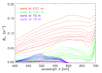
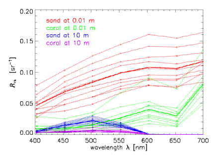
Now consider subsets of the entire database that define various classes of spectra. To be specific in the illustrative computations below, we chose four classes of spectra: for 10 sand and sediment spectra seen through 0.01 m of water, 10 coral spectra seen through 0.01 m of water, and the same sand and coral spectra seen through 10 m of the same water. The water IOPs were based on measurements of the very clear water in the Bahamas. The sand and sediment spectra range from clean ooid sand to heavily biofilmed, darker sand. The coral spectra are different species of corals. Figure 1 shows the individual spectra in these four classes. To minimize the array sizes for the printout of Table 1 below, we subsampled the spectra to wavelengths of 400, 450, ..., 650, 700 nm, so that . The subsampled spectra are shown in Fig. 2.
These spectra are obviously correlated in wavelength. The amount of correlation between one wavelength and another is quantified by the covariance and correlation matrices, which are computed as follows. Let label the class, with being the total number of classes (here 4). Class contains spectra (here, for each class). Then the mean or average spectrum for each class is defined by
| (2) |
where the sum is over the spectra belonging to class . In vector notation this is
| (3) |
The mean spectra for the example four classes are shown by the heavy lines in Fig. 2.
The elements of the class covariance matrices are defined by
| (4) |
expresses the covariance of the class spectra at wavelength with ; is the variance of the class spectra at . For remote-sensing reflectance spectra with units of , the units of are . If we arrange the spectrum column vectors for class in a matrix with the class mean removed,
| (5) |
then the covariance matrix for class can be compactly written as
| (6) |
The elements of the correlation matrix for class are defined from the class covariance matrix by
| (7) |
Table 1 shows the class covariance and correlation matrices computed by these equations for the four classes of spectra shown in Fig. 2.
Table 1. Covariance and correlation matrices for the four classes of spectra seen in Fig. 2. Wavelength 1 (400 nm) is at the upper left and wavelength 7 (700 nm) is at the lower right of each array. Units for are ; is non-dimensional.
These specific examples make it clear that
- For a given class, at one wavelength is highly correlated with at another wavelength, as expected.
- The covariance and correlation matrices are different for each class. These matrices depend not only on bottom type (sand vs coral) but also on bottom depth (and water IOPs, not explicitly shown here). In other words, the wavelength covariances carry information about both bottom type and water depth and IOPs.
Spectrum Matching vs. Statistical Classification
One metric for comparing two spectra is the simple Euclidean metric, which measures the squared distance (in units of ) between an image spectrum and each in the database:
| (8) |
The spectrum giving the minimum distance of all database spectra determines the closest match to the image spectrum . Note that this is not a statistical estimate in the sense that no probability model is involved. Note also that the image spectrum is being compared with every spectrum in the database, not just with pre-defined class mean spectra.
In traditional thematic classification, an image spectrum is compared only with the mean spectrum and “size”’ for each class, as expressed by the class mean and covariance . Here “size” is used in the sense that the variances and covariances in are larger when the spread of spectra is greater. Inspect, for example, the elements of for the class of sand at 0.01 m compared to sand at 10 m, for which the spectra are all much closer together (especially at blue and red wavelengths) and thus have smaller covariances. The class covariance matrix defines the size of the “swarm of points” surrounding the centroid (mean class spectrum) representing the class in K-dimensional space. The image spectrum is assigned to a particular class according to a statistical model (often based on the assumption of a multivariate normal distribution of the swarm of points) that determines the probability that the image spectrum belongs to a particular the swarm of points defining a given class. The class spectra (K-dimensional swarms of points) generally overlap, so that an unambiguous, non-probabilistic association of with a given class is not possible.
In maximum likelihood estimation (MLE; see Richards and Jia (1996) for an excellent discussion of this whole business), the distance metric is
| (9) |
where denotes the determinant of and denotes the inverse. and are of course pre-computed for each class before doing the spectrum matching. The image spectrum is assigned to the class m having the smallest value of . Note that now the image spectrum is compared only with the class mean spectra . The assignment of the image spectrum to a particular class is based on its closeness to the class mean and the spread of the “swarm of points” surrounding the mean, as described by the covariance matrix. This metric involves matrix multiplication, which is computationally expensive, but the number of classes is generally small, so in practice this may not be a problem.
It is often said that the incorporation of into the distance metric “removes the effect of correlations between wavelengths.” This interpretation of the effect of relates to the fact that covariance matrices are the foundation of principle component analysis (PCA; see Preisendorfer (1988)). In PCA the original independent, physical variables (here, the wavelengths) are transformed to obtain a new set of (generally unphysical) independent variables for which the data are uncorrelated. This transformation can be viewed as a rotation of the axes of the original, physical data space (here the wavelength axes used for plots in K-dimensional space) to generate new (generally unphysical) axes for which the data are uncorrelated.
If the class covariances are equal (or assumed to be equal), then is the same for each class and can be ignored. The MLE metric then reduces to the Mahalanobis distance metric,
| (10) |
where is the common value of . The image spectrum is then assigned to the class m having the smallest value of .
We have seen by the specific examples of Fig. 2 and Table 1 that the covariance matrices are different for different classes of the sort that are relevant for ocean-bottom remote sensing. Indeed, Table 1 shows that the elements of the can change by orders of magnitude as a function of water depth. This inequality of the for different classes precludes use of the Mahalanobis metric for classes as defined here. For the retrievals needed for shallow-water mapping of bottom type, MLE (or something else) would have to be used with a different covariance matrix for each class.
However, it is not at all clear how meaningful classes should be defined for simultaneous retrievals of bottom type, water column IOPs, and bottom depth. Should one class be “sand spectra at 5.25 m depth with a particular set of water absorption, scattering, and backscatter spectra,” and another class be “sand spectra at 5.25 m depth with the same absorption and scattering spectra but a different backscatter fraction,” and another class be “sand spectra at 5.50 m with the first set of IOPs,” and then another class be “sea grass spectra at 7.50 m with yet another set of IOPs,” and so on? If so, then the number of classes quickly becomes as large as the number of depths, IOP sets, and pre-chosen classes of bottom type (sand, coral, sea grass, etc.). A database generated as previously described easily could have hundreds or thousands of classes (a database often has 50-100 bottom depths, several dozen to several hundred sets of IOPs, and more than 100 bottom reflectance spectra). With such a large number of classes, the validity of doing traditional thematic mapping becomes uncertain, not to mention the additional computational costs involved with the matrix multiplications.
Clearly spectrum matching for shallow-water applications addresses a much more complicated problem than classic terrestrial thematic mapping, which corresponds to retrieval of bottom type if there were no water present, i.e. no simultaneous retrieval of depth and IOPs. Because of the greater complexity of the oceanographic retrieval problem, and because of the difficulty in defining meaningful classes, shallow-water spectrum matching does not use statistical classification techniques such as MLE. The spectrum matching approach of Mobley et al. (2005) does not compare an image spectrum to a class mean spectrum. In that technique, an image spectrum is compared to every spectrum in a database to find the closest match by the chosen (Euclidean or some other) metric, which is appropriate in this case. In a manner of speaking, each database spectrum is a separate class corresponding to a particular depth, bottom reflectance spectrum, and set of IOPs. In such a situation (only one member in each class) the covariance matrix is undefined.
Moreover, for the present problem it is not even desirable to remove the effects of wavelength correlations, as can be done with the MLE or Mahalanobis metrics, because the wavelength correlations carry information that is critical to separating depth and IOPs effects from bottom type effects.
The spectrum-matching approach of Mobley et al. (2005) for shallow-water benthic mapping therefore avoids defining predetermined classes and finds the closest match from the entire database. This gives the highest possible resolution (in depth, bottom type, and water IOPs) of retrievals. This approach retrieves a particular bottom reflectance spectrum (which represents a particular bottom type), not just a generic bottom type such as sand or coral. If the user later wishes to group the particular spectra for the retrieved bottom types into broader classes such as corals vs. sediments, or to group the retrieved IOPs into low, medium, and high absorption bins, for example, then that is easily done from the full-resolution retrieval.
 See comments posted for this page and leave your own.