Page updated:
May 19, 2021
Author: Curtis Mobley
View PDF
The Luminance Transfer Equation
The Radiative Transfer Chapter derived the scalar radiative transfer equation (SRTE), Eq. (3) of the Scalar Radiative Transfer Equation page:
This equation governs the propagation of unpolarized monochromatic radiance at a particular wavelength in a one-dimensional absorbing and scattering medium.
The question now arises: Is there a similar equation for the propagation of luminance? It is to be anticipated that a luminance transfer equation may be more complicated than the SRTE because it of necessity must involve all visible wavelengths and the response of the human eye.
The Luminance Transfer Equation
To develop a luminance transfer equation, multiply Eq. (1) by the photopic luminosity function and integrate over all visible wavelengths. Let denote the range of wavelengths for which . The term on the left hand side of the SRTE then becomes
where the luminance is defined by Eq. (1) of the Photopic Luminosity Function page:
The first term on the right hand side of the SRTE becomes
This term does not give a product of an integral over wavelength of the beam attenuation coefficient times the luminance. However, we can rewrite this term as
The term in braces is a radiance-weighted integral of the beam attenuation coefficient times the photopic luminosity function . If we define the photopic beam attenuation coefficient as
| (2) |
then the term of the SRTE maintains the same form, , in the luminance transfer equation.
A similar treatment of the path radiance term of the SRTE leads to a definition for the photopic volume scattering function:
| (3) |
The source term in the SRTE leads to a photopic source term:
Collecting the above results gives the desired luminance transfer equation:
This equation governs the propagation of broadband luminance as seen by the human eye in a one-dimensional absorbing and scattering medium. Equation (4) is the basis for the classical definition of contrast as used in visibility studies.
Dependence of on the Ambient Radiance
It is important to note that the photopic beam attenuation coefficient as defined in Eq. (2) depends on the ambient radiance distribution, hence on direction , even though the beam attenuation is an inherent optical property (IOP) that does not depend on the ambient radiance or direction. Moreover, meets the definition of an apparent optical property as defined on the Apparent Optical Properties page: it depends on the IOPs of the medium (here the beam attenuation ) and on the ambient radiance distribution, and it is insensitive to external conditions (e.g., rescaling by a multiplicative factor does not change the value of ). The same holds true for the photopic volume scattering function defined in Eq. (3) and for any other IOP. Thus, in going from a monochromatic radiative transfer equation to a luminance transfer equation, inherent optical properties become apparent optical properties. This is the penalty to be paid for going from an equation for monochromatic radiance as measured by instruments to an equation for luminance observed by a human eye.
However, in practice, there seems to very little dependence of on the ambient radiance (as would be expected for a “good” AOP). The left panel of Fig. 1 shows the beam attenuation for a simulation of homogeneous Case 1 water with a chlorophyll concentration of (obtained using the new Case 1 IOP model in HydroLight). The Sun was at a zenith angle of in a clear sky, which gives a transmitted solar beam of about 29 deg in the water; that beam will lie in the HydroLight quad centered at . The right panel of Fig. 1 shows the radiance at 10 meters depth looking in four directions: looking upward into the Sun’s transmitted beam, looking in the nadir and zenith directions, and looking horizontally at right angles to the solar plane.
The spectra in this figure were used to compute the photopic beam attenuation via Eq. (2). The values are all close to , which is close to the beam attenuation at the peak of the photopic luminosity function: .
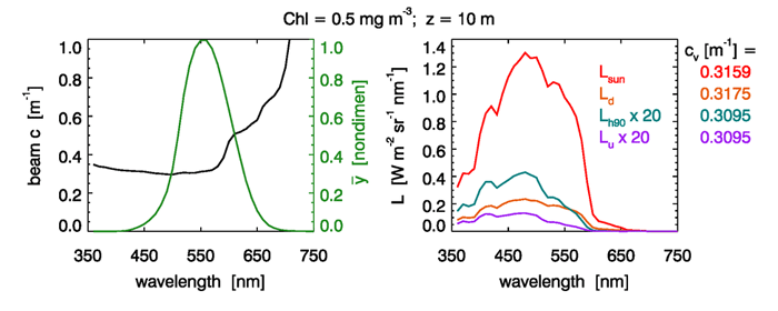
Figure 2 shows the corresponding results for a chlorophyll concentration of and a 5 m depth. Again, the four different radiances give the same to within a fraction of a percent, and these values are within one percent of the beam attenuation value .
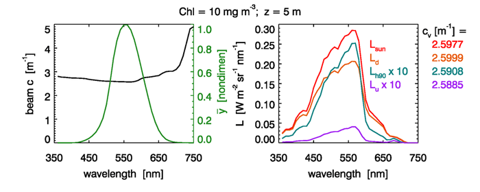
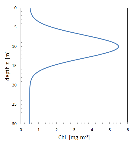
Figure 3 shows a chlorophyll profile consisting of a background value of plus a Gaussian that gives a maximum value of at 10 m depth. For this profile, an observer at 5 m depth looking upward would be looking into low-chlorophyll water, and looking downward would be looking into high-chlorophyll water. An observer at 10 m depth looking horizontally would be looking into high-chlorophyll water, but looking upward or downward would be looking into lower chlorophyll, clearer water. It might be supposed that the different IOPs ( values in particular) would give radiances that might give significantly different values for the different viewing directions at a given depth.
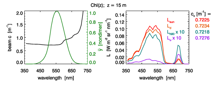
However, this is not the case. Figure 4 shows the radiances seen by an observer at 15 m depth. Again, the values differ by only about one percent from the value of . The same holds true at other depths (not shown).
Exhaustive simulations have not been made, so it might be possible to create a contrived water body for which the photopic beam attenuation would be significantly different for different viewing directions, and for which would be significantly different from . However, the above simulations indicate that in many situations of practical interest, there is little dependence of on viewing direction, and that is within a percent or so of the beam attenuation at the 555 nm wavelength of the maximum of the photopic luminosity function.
These simulations are consistent with the results of Zaneveld and Pegau (2003), who found that the beam attenuation coefficient at 532 nm (excluding the water contribution) is a good proxy for the photopic beam attenuation.
 See comments posted for this page and leave your own.