Page updated:
May 7, 2021
Author: Curtis Mobley
View PDF
Counting Photons
[Bryan Monosmith, Jeremy Werdell, and Curtis Mobley contributed to this page.]
The foundation of ocean color remote sensing is sunlight that has entered the ocean, been transformed through absorption and scattering by the myriad constituents of the water body, and then been scattered out of the ocean and into a detector. It is worthwhile to consider how many photons going through this process are actually available for detection by a satellite sensor. An order-of-magnitude calculation suffices to identify many of the engineering constraints on the design of an ocean color sensor.
Radiance from the Sea Surface
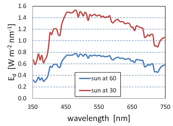
Figure 1 shows that the downwelling spectral plane irradiance onto the sea surface on a clear day is of order at visible wavelengths. Most (90-98%, depending on sun zenith angle and wind speed; e.g. Light and Water Figs. 4.11-4.13) of this irradiance enters the ocean. In-water irradiance reflectances are typically in the 0.01 to 0.05 range, depending on the water constituents and wavelength ( can reach 0.1 in very turbid, highly scattering waters).
Suppose that of downwelling plane irradiance of magnitude entering the ocean is backscattered into upward directions. If this upwardly scattered light is isotropically scattered into the of the upward hemisphere, then the upwelling isotropic radiance just below the sea surface would be
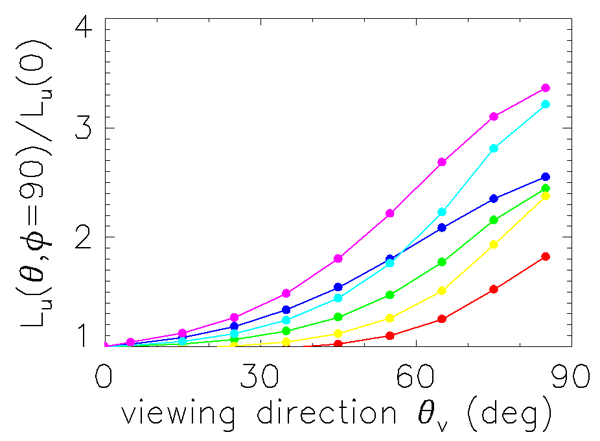
For ocean waters the upwelling radiance is not isotropic. Just below the sea surface, upwelling radiance within 30 deg of the zenith (the angles relevant to remote sensing) is less than the radiance in more nearly horizontal directions by a factor of two or three, as shown in Fig. 2. Thus the above value for isotropic scattering can be reduced by a factor of roughly to estimate the underwater radiance in near-zenith directions.
A beam of this radiance just below the sea surface will be reduced by a factor of when passing through the sea surface. Here is the water-to-air radiance transmittance, which is close to 1 for directions relevant to remote sensing, namely directions within a few tens of degrees of the zenith. is the water index of refraction. The water-leaving radiance is then roughly
Atmospheric transmittance is 0.7 to 0.95 at visible wavelengths, so most of the water-leaving radiance will be transmitted to the top of the atmosphere (TOA), where it can be detected by a satellite. However, along the way, atmospheric scattering of solar radiation into the beam will add typically 10 to 20 times as much radiance to the beam. The TOA radiance seen by a satellite would then be of order . Typical open-ocean TOA radiances for the MODIS sensor are in the range of 0.01 (red wavelengths) to 0.08 (blue wavelengths) .
Photons Detected
Now that we have the radiance detected at the satellite, we can compute the numbers of photons collected and consider the related engineering matters. We start by computing the number of detected photons that come from a patch of sea surface in 1 second of observation time. For specific numbers, the MODIS sensors have the following characteristics:
| Physical quantity | value |
| altitude | 705 km = |
| off-nadir viewing angle | 20 deg |
| slant range | 750 km = |
| sensor aperture radius | 89 mm = 0.09 m |
| band width | |
| optical efficiency | OE = 0.6 |
| quantum efficiency | QE = 0.9 |
The slant range is the distance from the satellite to the observed point on the ocean surface along the line of sight, which is taken here to be 20 deg off nadir. The optical efficiency is the fraction of light incident onto the sensor fore-optics that eventually reaches sensor material itself; the losses are due to reflections from lens surfaces or diffraction gratings, absorption by filters, etc.
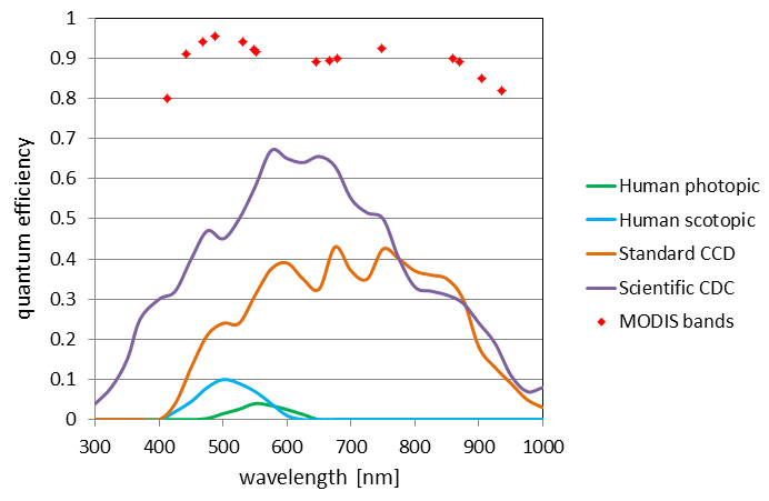
The quantum efficiency is the fraction of photons reaching the sensor material that actually results in a signal, e.g., by the generation of a photo-electron. Figure 3 shows the quantum efficiencies of typical sensors. The ”standard CCD” curve is for CCDs like those used in consumer-grade video cameras. “Scientific CCD” is for a much more expensive “science grade” CCD. The MODIS curve shows what is achievable if your budget is almost unlimited. The bottom curves are for the human eye. The human eye has a maximum QE of only a few percent for color (photopic) vision and 10% for night-time (scotopic) vision. It thus seems that evolution has given us eyes that are adequate for finding food and avoiding tigers, and even for reading websites, but which are shockingly inefficient from an optical engineering standpoint. (This figure gives another refutation of “intelligent design” for the human eye. The intelligent design in this figure was done by the physicists and optical engineers working on the CCD and MODIS sensors.)
The solid angle of the sensor as seen from the Earth’s surface is
The power detected by the sensor coming from a square meter of the ocean surface is
[This equation has been written for viewing the satellite from the sea surface. We could also take the viewpoint of the satellite viewing the earth. In that case, the relevant solid angle would be that of the pixel as seen from the satellite, and the area factor would be that of the sensor aperture. The throughput, or etendue, of an optical system is
which shows that these viewpoints are equivalent.]
If we assume a wavelength of 550 nm, the corresponding number of photo-electrons released in the detector in time is
where is Planck’s constant and is the speed of light.
These 6800 electrons are for the total TOA radiance in this green band. As previously noted, the TOA radiance is typically 90% atmospheric path radiance, in which case only 680 of these electrons correspond to the water-leaving radiance from a square meter of the sea surface.
Kepler’s third law of planetary motion and Newton’s law of gravity give the relation between a satellite’s orbital period and the radius of its orbit:
where is Newton’s gravitational constant and is the mass of the earth. For a satellite at altitude 705 km above the earth (whose mean radius is 6731 km), this gives a period of 6385 s. This corresponds to a speed of relative to the ground. The time required for the satellite to travel 1 m is then . For 1 m spatial resolution, this short exposure time reduces the number of detected photons by a factor of compared to the 1 s collection time computed above. Thus the number of water-leaving photons collected during the time the satellite passes over the area is only 0.093. Alas, the actual situation is even worse because the sensor is not collecting light from just one pixel, but from perhaps 1000 pixels as the sensor either scans back and forth or rotates to observe a wide swath to either side of the satellite nadir point. Thus, in the time required for the satellite to move forward by 1 m, the sensor must collect photons from 1000 pixels, reducing the number for each to roughly 0.0001 photoelectrons per pixel. Collecting only 0.0001 photoelectrons per pixel would not yield a very good image.
These physical and orbital constraints show one reason why orbiting satellites do not obtain meter-scale ocean color imagery: There simply are not enough photons leaving the ocean surface from a square meter of area to form an image. Many more photons must be collected, and there are several ways to do this:
- View a larger surface area, which both increases the number of photons leaving the surface and allows for longer integration times.
- View the surface area for a longer time, e.g., from a geostationary satellite that can stare at the same point for very long times (but a geostationary satellite has an altitude of 36,000 km, which makes the solid angle much smaller).
- Get closer to the surface, e.g. by using an airborne sensor flying at a few kilometers above the sea surface. This greatly increases the solid angle of the sensor and allows for longer integration times for a slowly flying aircraft.
- Increase the bandwidth.
- Increase the aperture of the receiving optics.
- Use multiple detector elements to observe the same ground pixel nearly simultaneously, either on the same or successive scans, and then combine the photons collected from the different sensors.
Suppose, as is typical of ocean color sensors such as MODIS, that we image a area of ocean surface. This increases the number of photons leaving the imaged pixel by a factor of and the integration time by a factor of (the increased time for the satellite to travel 1 km rather than 1 m). The sensor now collects 93,000 photoelectrons from the water-leaving radiance. The total number of TOA photoelectrons, including the atmospheric path radiance, would be roughly ten times as large, about . In practice, this number will be less because of the duty-cycle time of the sensor: a rotating sensor will be viewing the ocean only about one-third of the time, and a scanning sensor will require time to stop and start each scan. Nevertheless, we can still collect roughly photoelectrons for each pixel, of which correspond to water-leaving radiance.
The signal to noise ratio, SNR, is given in general by
where the signal is the number of photoelectrons counted. The terms in the denominator represent the noise terms for the photoelectrons (PE), dark current (DC), sensor read-out (RO), and quantization (QN). Dark current noise results from the spontaneous emission of photoelectrons within the sensor, read-out noise comes from the sensor’s analog front-end electronics when the collected photoelectrons are read from the sensor, and quantization noise comes from uncertainty when the analog signal is digitized. (Writing the total noise as the square root of the sum of the individual noise terms squared assumes that the individual noise processes are uncorrelated.) The number of photoelectrons counted during a given time interval is described by a Poisson probability distribution, for which the noise is the standard deviation of the distribution, which in turn equals the number of photoelectrons counted. The emission of dark current photoelectrons is also a Poisson process. The SNR can thus be written
Assuming no dark current or other noise, this gives an SNR of
for the number of photoelectrons estimated above. The actual SNR will be somewhat less due to dark current, read out, and quantization noise. The MODIS sensor has SNR requirements of 750 to 1000 for various bands, so we have achieved the approximate number of photons needed at the sensor.
These simple estimates illustrate the severe constraints on the design of any ocean color sensor. In practice, the engineering of a satellite ocean color sensor requires great sophistication to achieve the needed SNR.
 See comments posted for this page and leave your own.