Page updated:
March 14, 2021
Author: Curtis Mobley
View PDF
Empirical Line Fits
[Contributors to this page include Richard Zimmerman and Victoria Hill of Old Dominion University, who made the field measurements and developed the ELFs; Paul Bissett (then at WeoGeo, Inc.), who provided the WV2 image; and Curtis Mobley.]
The “black-pixel” technique discussed on the Aerosols page works well in many open-ocean situations, but it is not applicable if the water-leaving radiance is not very close to zero at the near-IR wavelengths used to model the aerosol scattering. This can occur for two reasons. First, if the water contains mineral particles, these highly scattering particles can give a significant amount of water-leaving radiance even out to 1000 nm and beyond. Such particles are common in coastal waters because of inputs by rivers or sediment resuspension by strong currents. Second, if the water is clear and less than a meter deep, there can be significant water-leaving radiance due to bottom reflectance, especially for bright sand bottoms.
Case 2 and shallow waters are of great interest for reasons such as ecosystem management, recreation, and military operations, and such waters are often observed from aircraft with hyperspectral imaging sensors. New techniques have been developed for atmospheric correction of such imagery.
In general, we need an atmospheric correction technique that
- works for any water body (Case 1 or 2, deep or shallow),
- works for any atmosphere (including absorbing aerosols), and
- does not require zero water-leaving radiance at particular wavelengths (no black-pixel assumption).
Two basic atmospheric correction methods have been developed in response to these needs. The first of these is a correlational technique called empirical line fitting, which is discussed on this page. The second, discussed on the next page, uses atmospheric radiative transfer calculations.
The essence of the empirical line fit (ELF) technique is as follows:
- Make field measurements of the remote-sensing reflectance [or water-leaving radiance , or non-dimensional reflectance , or whatever is needed by your retrieval algorithms] at the same time as the image acquisition and at various points within the imaged area.
- The measurements at various points in the imaged area are then correlated with the at-sensor measurements for the image pixels viewing the stations where was measured. The at-sensor spectra can be in any units, e.g. radiance or digital counts. The correlation functions that convert at-sensor spectra to sea-surface values are the empirical line fits. A different ELF is obtained for each wavelength.
- Assume that the atmospheric conditions, surface waves, and illumination are the same for every pixel in the image.
- The ELFs, which were developed from a few image pixels, are then used to convert the at-sensor measurements to sea-level spectra for every pixel in the image
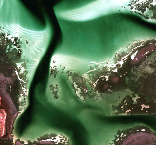
To illustrate how this process works, ELFs were developed for a DigitalGlobe WorldView-2 image of shallow Case 2 waters in St. Joseph’s Bay, Florida, USA. WorldView-2 (WV2) is a commercial satellite that provides high spatial resolution (approximately 2 m pixel size), 8-band multispectral imagery. Figure 1 shows an RGB image of this area, created from WV2 bands 5 (656 nm), 3 (546 nm) and 2 (478 nm) for the red, green, and blue values. The area includes some dry land (at the lower left of the image), areas of dense bottom vegetation (reddish color in this image), clean sand bottom (white to green, depending on depth), and an optically deep channel (darkest area). These Case 2 waters are optically deep (the bottom cannot be seen) for depths greater than about 3 m.
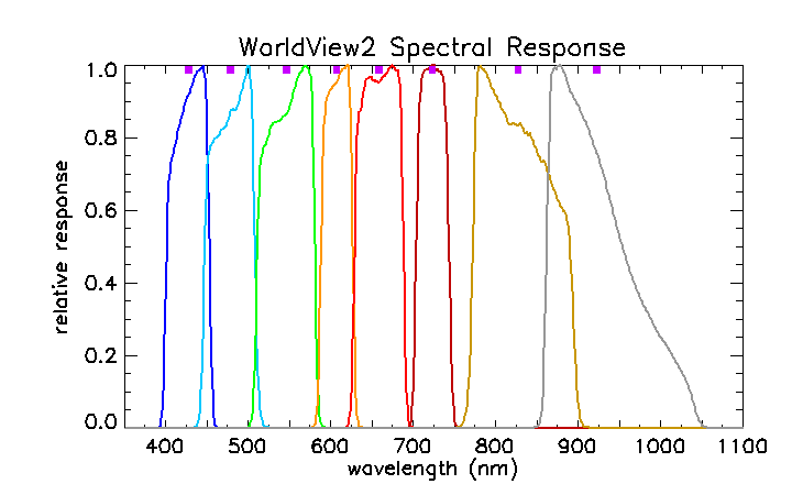
Hyperspectral measurements were made from a small boat at 10 stations in St. Joseph’s Bay. Those spectra were then weighted by the WV2 spectral response functions for each of the 8 bands to obtain multispectral spectra that correspond to the 8 WV2 bands. Figure 2 shows the relative spectral response of the 8 WV2 bands. Thus , the equivalent of corresponding to WV2 band , is obtained from
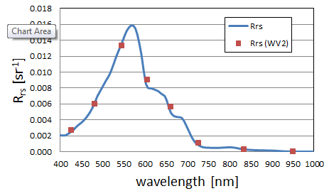
where is the spectral response function for band as seen in Fig. 2. Figure 3 shows one of the measured hyperspectral spectra and the corresponding values for the WV2 bands.
Each of the WV2 image pixels “looking” at the 10 ground stations was then used to correlate the WV2 top-of-the-atmosphere (TOA) band values in digital counts (DC) with the sea-level values for each of the 8 bands. Figure 4 shows the results for WV2 band 3, which is centered at 546 nm. The best-fit line to these 10 points is the ELF for this wavelength band. In this example, the ELFs convert the TOA measurements in digital counts to sea-level values in units of . These ELFs, obtained from only 10 points, are then applied to every pixel in the image. Note that the measured spectra correspond to different water IOPs, bottom depths, and bottom types, but the atmospheric conditions and viewing geometry (and resulting atmospheric path radiance) are assumed to be the same at each ground station.
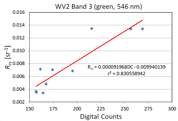
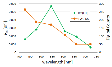
Figure 5shows an example WV2 TOA spectrum (excluding the two bands in the IR) and the corresponding sea-level spectrum obtained from the 6 ELFs. Note for band 3, for example, that the TOA value of 170 DC is converted to an value of 0.0057 , in accordance with the ELF of Fig. 4.
The advantages of the ELF technique are
- The ELFs account for atmospheric path radiance for any atmospheric conditions, without the need to know what these conditions are. No atmospheric measurements are needed.
- The technique works for shallow or Case 2 waters, for which is not zero.
- The technique works for any sun and sensor geometry, or sensor altitude (airborne or satellite sensors).
The disadvantages of the ELF technique are
- Field measurements of must be made at the time of image acquisition, which is labor intensive and often impossible.
- A set of ELFs is valid only for the one image used for their development. ELFs for one image cannot be applied to a different image of the same area, or to a different area, because the atmospheric conditions, or sun and viewing geometry, will differ for other locations and times.
- The field measurements always contain errors, which introduces an unknown amount of error into the ELFs, hence into the final spectra.
- The same ELFs are applied to all image pixels, even though the atmospheric and water conditions and viewing geometry may vary from one part of the image to another. (For airborne sensors, the viewing geometry and atmospheric path radiances can vary greatly from one part of an image to another.)
 See comments posted for this page and leave your own.