Page updated:
March 13, 2021
Author: David Bowers
View PDF
Optical Properties of Shelf Seas and Estuaries
The majority of the literature on ocean optics has concentrated, understandably, on the majority of the ocean. For most people, however, their nearest stretch of salt water is a shelf sea: water lying on a continental shelf and less than 200 metres deep. Shelf seas occupy 6-8% (depending on definition) of the surface area of the world ocean but contain about 16% of the world’s phytoplankton biomass. These seas are also rich in mineral particles stirred up from the sea bed by tides and waves and dissolved organic matter brought in by rivers. The waters are coloured green or blue-green by the mixture of pigments in phytoplankton, coloured dissolved organic matter (CDOM) and minerals. The optical properties of phytoplankton and their pigments are dealt with in other sections of this document and in several excellent textbooks on marine optics (e.g. Kirk (1994)) but CDOM and mineral particles have their own special features in shelf seas and deserve an account of their own.
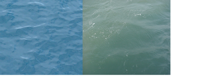
Shelf seas are considered to be optically complex because the CDOM and mineral particles can make a significant (or even the dominant) contribution to water colour and brightness. Both CDOM and mineral particles absorb light most strongly in the blue part of the spectrum and so, when added to water (which absorbs mostly red light), they produce a green colour which is easily confused with the effect of phytoplankton pigments. For this reason, satellite remote sensing algorithms for chlorophyll regularly fail in shelf seas in the sense that they over-estimate the chlorophyll content. In remote sensing terms, these waters are classified as Case 2 (Morel and Prieur (1977)) as distinct from Case 1 open ocean waters. The mineral particles suspended near the sea surface are also excellent scatterers of light. Because of this, shelf seas appear bright (highly reflective) when viewed from space.
CDOM in Shelf Seas
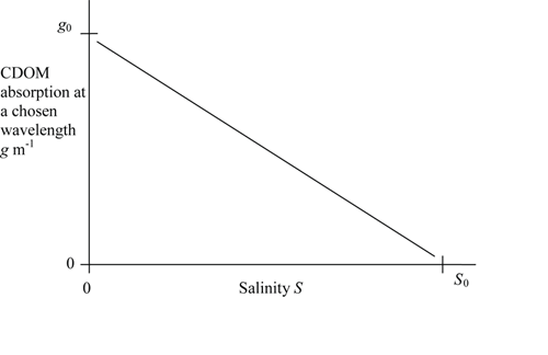
Coloured dissolved organic matter (CDOM, also called yellow substance or gelbstoff) is produced when organic material decays. In the open ocean, the main source of CDOM is from the decay of phytoplankton and there is sometimes a correlation between the concentration of chlorophyll and the concentration of CDOM which is helpful in remote sensing chlorophyll in these waters. Shelf seas in temperate latitudes, however, receive significant fresh water input from the land and this brings with it CDOM produced by the decay of terrestrial plants. This can be the main source of CDOM in shelf seas, particularly near the coast, dominating the marine production of CDOM. In these circumstances it is not reasonable to expect there to be a correlation between CDOM and chlorophyll concentrations in shelf seas. As the fresh water runoff mixes with sea water, the land-produced CDOM is diluted. This leads to a negative correlation between CDOM and salinity of the form
| (1) |
where is the CDOM concentration at a point where the salinity is , is the concentration in the source water (where the salinity is zero) and is the gradient of a plot of against . Since CDOM is often measured optically, the ’concentration’ of CDOM, and may be expressed as its absorption coefficient of a filtered water sample at a chosen wavelength (Kirk (1994)). An example of the relationship between CDOM absorption and salinity in an estuary is shown in Fig. 2.
Effect of variations in source concentration
A linear relationship between CDOM and salinity (obeying Eq. (1)) is observed surprisingly often (although not always) in shelf seas and estuaries. This is taken to indicate ’conservative mixing’, that is the CDOM mixes passively with water in the same way as salt. This is surprising, since it is known that CDOM is consumed in water (by bacteria; it is also destroyed by sunlight) and it is produced by the decay of organic matter at sea. The observation of a linear relationship is also surprising because the concentration in the source water can be expected to change with time. The intercept of a plot of CDOM against salinity at zero salinity is not fixed but moves up and down in response to seasonal and other changes in CDOM production at the source.
Bowers and Brett (2008) have analysed the effect of variations in source concentration on the CDOM-salinity relationship in shelf seas and estuaries using a simple box model. They found that in a water body with a short flushing time compared to the timescale of the source variation (for example, a small body of water such as an estuary), the concentration of CDOM can ’keep up’ with the fluctuations in the source and so the linear relationship between salinity and CDOM is maintained, although the slope changes with time (as illustrated in Fig. 2). In larger water bodies, such as a bay or a gulf, the slow response time of the water body buffers it against rapid changes in the source concentration, so again there is a linear relationship between salinity and CDOM, this time with a fixed slope set by the long term mean concentration of CDOM in the source.
Using CDOM to trace water masses in shelf waters
A useful technique in classical physical oceanography is water mass analysis, which uses temperature-salinity diagrams to identify the source of water in the ocean and mixing between different sources. This technique does not work in shelf seas (nor in the surface waters of the ocean) because temperature is affected too much by the heat flux through the sea surface. Instead, Stedmon et al. (2010) have proposed using CDOM instead of temperature to trace water masses in shelf seas. Water samples are placed on an x-y plot which has CDOM concentration (i.e. absorption at a chosen wavelength) on one axis and salinity on the other, that is a diagram like Fig. 2. If sources can be identified by their characteristic salinity-CDOM value (and for a large water body, the long term mean values can be used - see above), then the proportion of water in a given sample from either two or three sources can be established. Stedmon and co-workers, applied their technique to the Baltic-North Sea transition zone. The three end-member water masses where the German Bight, the Baltic outflow and the central North Sea. The method gave believable results for the distribution of these 3 water masses in the study area. The method assumes that CDOM behaves conservatively. Stedmon et al. (2010) tested this assumption by using a third variable: the spectral slope of CDOM absorption, and concluded that the CDOM was behaving conservatively.
Remote sensing of CDOM and salinity
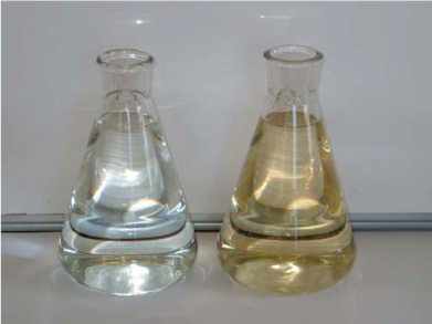
CDOM in coastal waters acts as a dye (see Fig. 3) producing a colouration which can be seen from space. In water in which CDOM is the principal optical component this means that it is possible to measure CDOM concentration using ocean colour and, because of the relationship between CDOM and salinity, this technique can also be used to map salinity in coastal water bodies. A number of empirical relationships between water colour and CDOM have been proposed (Kutser et al. (2005); Del Castillo and Miller (2008)) but it is possible to arrive at a theoretically sound relationship using the fact that CDOM is a strong absorber in the blue and a weak one in the red.
The reflection coefficient at a given wavelength just below the water surface is proportional to the ratio of the backscattering to absorption coefficient at that wavelength (Morel and Prieur (1977)). Assuming that (i) absorption in the red is dominated by water, (ii) absorption in the blue is due to CDOM and water and (iii) the ratio of backscattering coefficients in the red and the blue is constant, it is possible to write an expected relationship between CDOM absorption in the blue and a ratio of reflection coefficients of the form:
| (2) |
Where is the absorption coefficient of CDOM at 440nm (a proxy for its concentration), is the reflection coefficient in the red and the reflection coefficient at another (shorter) wavelength. and are constants provided CDOM is the predominant influence on water colour. Binding and Bowers (2003) found a good (R2=0.94) fit for this expression against observations for , , , . They used this expression to map surface CDOM concentrations in the Clyde Sea in Scotland and to derive salinity using the known relationship between CDOM and salinity in the Clyde.
The application of water colour to derive CDOM concentration and salinity remotely is most appropriate in estuaries where the strongest signal is to be found. Unfortunately, the colour of the water in an estuary is also likely to be influenced by suspended particles (including mineral particles), although it may be possible to correct for this if the optical properties of the particles are known.
Suspended Mineral Particles in Shelf Seas
The combination of shallow water and high energy input (through waves and tides) in shelf seas means that mineral particles are lifted off the sea bed and mixed throughout the water column. The particles collide and stick together to form flocs. This process is particularly important during and after the spring bloom when there is plenty of organic material in the water to help the flocculation process (the organic material acts as a ’glue’ to hold the flocs together). Since flocs tend to have a higher settling speed than the constituent particles this flocculation process after the spring bloom is important in making surface waters in shelf seas becoming clearer.
Flocs are considered to be fairly delicate objects, easily broken up in the turbulent shear involved in collecting a water sample for instance. For this reason, the most reliable measurements of floc properties are made in situ using instruments which do not disturb the flocs. Because flocs cannot withstand turbulence it has been suggested that the largest flocs will have the same size as the smallest turbulent eddies, a size known as the Kolmogorov microscale. It is implied that other properties of the particle size distribution, such as the mean particle size, will change as the turbulent microscale changes and the largest flocs adjust to follow this. The Kolmogorov microscale depends on the rate of dissipation of turbulent kinetic energy. In a tidal sea this will fluctuate with the tide, being largest at times of slack water. There is growing evidence that the particle size in shelf seas responds to these changes and that the mean particle size at slack water can be several times greater than that at maximum tidal flow. This will have interesting implications for the optical properties of shelf seas and estuaries.
How exactly is it best to imagine the passage of light through a floc? Is it best to think of the floc as a single particle with uniform properties (an average of the particles composing the floc), or is the floc better described as a number of separate mineral pieces (with relatively high refractive index) embedded in a matrix of low refractive index organic material? Boss et al. (2009c) have described experimental and theoretical results that suggest that an optical model allowing for the complexity of the floc performs better than one that assumes that flocs are solid homogenous spheres, but the exact nature of the best model to use remains an open question.
Measuring the mass concentration of mineral particles
The concentration of mineral particles is measured by filtering a known volume of sea water through pre-weighed and pre-combusted GF/F filters (nominal pore size ). The filters are then combusted in an oven at for 3 hours to remove organic material, cooled and weighed again.
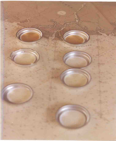
Light absorption by mineral particles
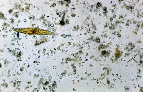
The absorption coefficient of mineral particles suspended in seawater can be measured directly using filters such as those shown in Fig. 5. The filters are placed, while wet, on a microscope slide and the slide is placed over the exit port of a spectrophotometer (the filter pad method). The optical density (OD) of the filter plus particles is recorded as a function of wavelength and the OD of a blank wet filter is subtracted. In calculating the absorption coefficient of the particles, allowance is made for the increase in the pathlength of the light through the particles and the filter produced by deviation of the light as it passes through the particles. The absorption coefficient of particles can also be measured in situ by measuring total absorption and subtracting the component due to water, organic material and CDOM.
The general shape of the absorption spectrum of mineral particles is one of exponential decay with increasing wavelength, often with a small ’bump’ at 500 nm. It appears that the absorption coefficient may not necessarily tend to zero in the near infra-red. The specific absorption spectrum of mineral flocs can therefore be represented by the following equation which includes the possibility of a non-zero absorption c1 at long wavelength:
| (3) |
Here, is the concentration-specific absorption coefficient of mineral particles (i.e. absorption per unit mass concentration, units ), is wavelength and is a reference wavelength. Bowers and Binding (2006) suggested mean values of , (for a reference wavelength of 443 nm) and based on their own measurements and those in the literature. There is no reason to suppose that the absorption spectrum of mineral particles should be the same from place to place and indeed variations in these coefficients are observed, but the slope parameter , in particular appears to be fairly tightly constrained.
Light scattering by mineral particles
There is no equivalent to the filter pad method for measuring light scattering by mineral particles. Scattering coefficients are instead measured at sea using instruments specifically designed for this purpose. Scattering coefficients measured in this way generally increase with the concentration of mineral particles, the rate of increase is the concentration-specific scattering coefficient for mineral particles . Specific scattering coefficients (units ) are observed to be rather flat spectrally and to vary over at least an order of magnitude in the range: .
There is some evidence that increases as the water becomes more oceanic and less coastal. Babin et al. (2003a) have suggested this is because of changes in particle density. Inshore particles tend to be more mineral in content and of higher density. They therefore can be expected to have a smaller cross sectional area per unit mass. A full appreciation of the variation of the specific scattering coefficient includes consideration of particle size as well as density and we turn to this in the next section. Even at the lower end of the range of , mineral particles are more likely to scatter light than absorb it. A typical value of at 555 nm is , therefore photons of this wavelength will be scattered at least 3 (and up to 30) times by mineral particles before they are absorbed by a mineral particle.
Theoretical Ideas About the Optical Properties of Mineral Particles
The probability that a photon will interact with a particle in suspension is proportional to the cross sectional area of the particle. For a suspension of identical particles, the absorption (or scattering) per unit cross sectional area is known as the absorption (or scattering) efficiency. For a suspension of spherical particles with a range of diameters (from to ) we can calculate the scattering (or absorption) coefficient by integrating the product of scattering (or absorption) efficiency and particle area over the range of sizes. For example, in the case of scattering by spherical particles with a range of sizes, the scattering coefficient can be written:
| (4) |
and there is an equivalent expression for the absorption coefficient. Here is the number of particles per unit volume in the size range to and is the scattering efficiency. Values of the scattering efficiency for spherical particles of given size and refractive index (both real and imaginary) are available from Mie theory or the simpler anomalous diffraction theory of van de Hulst (1957). It is often assumed that the size distribution of particles obeys a power law (or Junge) distribution, of the form:
| (5) |
where and are constants for a particular size distribution. A feature of equation 5 is that the number of particles rises rapidly as the size decreases. As a result, calculations based on equations 4 and 5 lead to the conclusion that optical properties are dominated by the large number of very small particles. For example, in the case of the scattering coefficient, it has been estimated that of light scattering by minerals is produced by particles smaller than (Babin et al. (2003a)). If this is the case, it would mean that much of the signal seen in visible band satellite images of shelf seas is produced by very small particles with low settling speeds. This would be an important conclusion for the interpretation of these images. However, there is no direct evidence that sub-micron sized particle exist in the numbers predicted by equation 5. Currently, measurements of particle numbers are limited to particles greater than a few microns in size. Furthermore, the flocculation process will tend to remove small particles and incorporate them in larger flocs (Flory et al. (2004); Boss et al. (2009c)).
Relationship Between Scattering and Mean Particle Size and Density
For any size distribution and shape of particle, equation 4 can be written as
| (6) |
where is the cross sectional area of particles in suspension in unit volume of water (units ) and is an effective scattering efficiency defined by
| (7) |
Equation 10 can then be written in terms of the bulk, measurable, properties of the particles as
| (8) |
where is the mass concentration of particles (dry mass per unit volume of water), is the particle density (dry mass of particle per unit volume of particle in situ) and is the Sauter diameter (volume of particles in situ per unit cross sectional area of particle in situ). It is possible to measure the volume of particles of different sizes in situ using laser diffraction (LISST) instruments and from these measurements, the Sauter diameter can be calculated. Combining these observations with the mass concentration of particles weighed on filter gives the particle density and therefore the validity of equation 8 can be tested. Bowers et al. (2010) found that 86 % of the variance in the scattering coefficient at stations along the west coast of Britain was explained by equation 8 with a constant . Since the concentration specific scattering coefficient of mineral particles this means that most of the variation in is explained by changes in both particle size and density. In fact, for the flocculated particles in the study by Bowers et al. (2010), the Sauter diameter changed by a factor of 3 and the density by a factor of 13, so it is mostly changes in particle density that are responsible for the variation in the specific scattering coefficient of mineral particles.
Relationship Between Absorption and Mean Particle Size and Density
We can write a similar equation to (8) for the absorption coefficient:
| (9) |
Where is an effective absorption efficiency and the other terms are as before. Unlike the scattering efficiency, for semi-transparent particles can be expected to vary with the particle size, since it is harder for photons to pass through large particles than small ones. A simple analysis of this problem proceeds as follows. The proportion of photons that pass through the centre of a particle of diameter composed of material with uniform absorption coefficient is . The proportion of photons that is absorbed within the particle is therefore . For small , and the proportion of photons absorbed within the particle increases linearly with the size of the particle.
For a suspension of particles of different sizes, Bowers et al. (2010) found that the effective absorption efficiency of particles in north-west European seas does increase with a measure of the mean size of the suspension—namely the Sauter diameter, . That is it is possible to write
| (10) |
where and are constants. At 555 nm a reasonable fit to the data at stations where was given by the expression
| (11) |
in which is expressed in microns. In the case of light absorption by mineral flocs, therefore, the absorption coefficient depends on the cross sectional area of particles in suspension (which depends on their size and density) and, in addition, the absorption efficiency depends on the size of the particles.
Remote Sensing of Mineral Particles in Shelf Seas
Mineral particles suspended near the sea surface colour the water and increase the reflection coefficient. Figure 6 shows a false colour SeaWiFS image of the north-west European shelf. The regions of bright, coloured water in the Irish Sea, the English Channel and the southern North Sea are mostly caused by mineral suspended sediments near the sea surface.
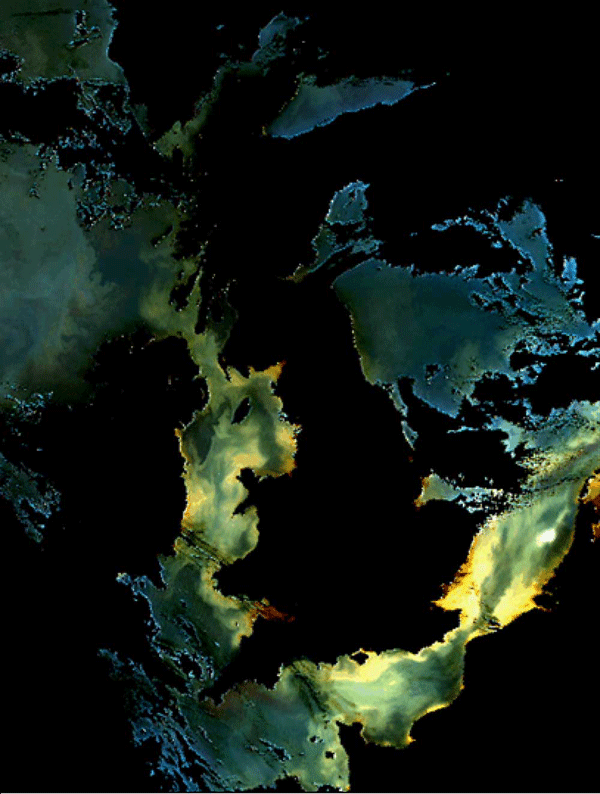
Quantitative interpretation of images such as figure 6 are based on the scattering and absorption properties of the mineral particles and of water itself. The most successful algorithms for predicting the concentration of mineral suspended sediments use the reflection coefficients in the red (Binding et al. (2005)) or, in the most turbid water, near infra-red parts of the spectrum (Doxaran et al. (2009)). Analysis of the vertical flux of photons in an absorbing ocean allows us to write the sub surface reflection coefficient as
| (12) |
(Morel and Prieur (1977), where is a factor that depends on solar elevation and sky conditions, is the backscattering coefficient and a the absorption coefficient. In water where the reflectance is mostly produced by mineral particles, equation 16 can be expanded as:
| (13) |
Where is the backscattering ratio , is the concentration of mineral particles, and are the concentration-specific scattering and absorption coefficients, respectively, is absorption by water and absorption by materials other than water and mineral particles. In the red and infra-red parts of the spectrum, the spectrum, absorption by water tends to dominate the denominator of equation 13 and, for low to moderate concentrations of mineral particles, the reflectance increases in proportion to , with a slope of . At higher values of , absorption by mineral particles becomes more important in the denominator and the reflectance tends towards an asymptotic value of . Choosing a wavelength at the red end of the spectrum where absorption by water is high extends the region where reflectance is proportional to concentration. Equation 17 forms the basis of most general quantitative algorithms for suspended sediments in shelf seas (Stumpf and Pennock (1989); Nechad et al. (2010).
In fact, as we have seen, and depend on the density and size of particles in suspension and changes in these properties, as well as of concentration, will produce changes in reflectance. What we are really seeing in images such as figure 6 is the cross sectional area of the particles in suspension. In order that remote sensing can be used to test and verify models of suspended particles (which predict mass concentration) we therefore need a better understanding of the relationship between particle mass and cross sectional area and that is a challenge for the near future.
 See comments posted for this page and leave your own.