Page updated:
March 13, 2021
Author: Emmanuel Boss
View PDF
Commonly Used Models for IOPs and Biogeochemistry
This page presents a number of commonly used models relating inherent optical properties (IOPs) and underlying biogeochemistry. Models for IOPs and AOPs are analytical expressions relating these optical variables to bio-geochemical parameters (e.g. chlorophyll, suspended matter) and/or describing their spectrum (relating their value at one wavelength with their value at another wavelength). Below is a “laundry list” of such models we assembled from the literature (see also Sosik (2008) for a recent compilation). This list is not exhaustive and we invite the readers to point our to us useful models they have developed or know of that we have not included. The users of such models are cautioned that they were developed from specific data sets and designed with specific applications in mind, which may or not be applicable to the conditions the user is applying them to. Also, it is important to note that the fit parameters will vary depending on the way a model is fit to the data (e.g. how uncertainties are assumed to behave) and the spectral range that is fit (e.g. Twardowski et al. (2004). Note that some of the observed variability in relationships is likely due to methodology in biogeochemical determinations (e.g. filtration), may be due to instrumental issues (e.g. spectral filters used (narrow vs. wide) and acceptance angle (e.g. Boss et al. (2009a). In addition, empirical relationships are likely to be biased to time and location of data used to derive them, and their generalization should be done with caution.
Colored dissolved organic material, CDOM
The CDOM absorption spectrum in the visible is most often described by an exponentially decreasing function:
| (1) |
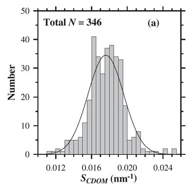
where is referred to as the spectral slope and is a reference wavelength. A theoretical explanation for this shape has been hypothesized by Shifrin (1988) as arising from a superposition of resonances of different molecular -bonds in the long organic molecules comprising CDOM. Single bonds, which are most abundant, will absorb short wavelength radiation while resonance of multiple bond, less abundant, absorb longer wavelength radiation. This explanation is consistent with the observation that small values of the spectral slope of CDOM, , are associated with higher molecular weight materials (e.g. Carder et al. (1989), Yacobi et al. (2003)). For visible wavelengths the most commonly used values of are near 0.014 , based on measurements by Bricaud et al. (1981) and others. However, the value of varies in the visible from 0.007 to 0.026 (e.g. Table 1 in Twardowski et al. (2004). Figure 1 shows the distribution of values observed by Babin et al. (2003b). Their data show a mean of with a standard deviation of 0.0020.
While Eq. (1) is the most frequent model of CDOM absorption, other models have been suggested, which may provide better fits to data (even when taking into account that fits improve as more free parameters are available in the fit, e.g. Twardowski et al. (2004). In particular, a constant is often added to the exponential fit:
| (2) |
What this constant represents is not clear. In some cases it is supposed to account for scattering by the dissolved component, however there is no reason to believe such scattering would be spectrally flat (see Bricaud et al. (1981) for in-depth discussion). It may account for bubbles in the sample.
Another model that has been found to work even better than the exponential model is the power-law model (e.g. Twardowski et al. (2004).
| (3) |
Models linking CDOM absorption to biogeochemical parameters
In estuaries and coastal waters, CDOM and fluorescence by dissolved organic matter (DOM) vary in correlation with DOM (e.g. Blough and Green (1995). Relationships are of the type:
| (4) |
for a variety of environmental samples as well as extracted fulvic and humic materials and where DOC has units of . When restricted to whole environmental samples (and including data from Vodacek et al. (1997)
| (5) |
Such relationships are not observed in open waters (Nelson and Seigel (2002)). However, the values of DOC observed in the open ocean (e.g. 48-68 , Nelson and Seigel (2002)), are of the similar magnitude as the intercept of – regressions ( Vodacek et al. (1997)) and hence represent, to a large extent, the surface pool of uncolored DOC. These relationships arise from end-member mixing between terrestrial and oceanic water masses and do not hold in coastal areas not strongly affected by river inputs and where CDOM sinks (e.g. photo-oxydation) affect CDOM concentrations significantly Blough and DelVeccio (2002)).
Between rivers and estuaries increases with increases in aromatic content and thus with lower CDOM spectral slopes (Blough and DelVeccio (2002)).
Prieur and Sathyendranath (1981) suggest the following model
| (6) |
Babin et al. (2003b) has also found a linear relationship between CDOM and Chl for European waters.
Non-algal particles
Similar to CDOM, the absorption of non-algal particles (NAP) is usually modeled with a decreasing exponential function (Yentsch (1962); Kirk (1980); Roesler et al. (1989), htmladdnormallinkBricaud et al. (1998)/view/references/publications/bricaud-et-al-1998):
| (7) |
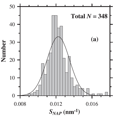
where is a reference wavelength and the spectral slope (independent of ). The mean slope () generally used to model is (e.g., Roesler et al. (1989), htmladdnormallinkBricaud et al. (1998)/view/references/publications/bricaud-et-al-1998). However, as always with data-derived parameters, there is variability in . Figure 2 shows the distribution of values observed by Babin et al. (2003b). Their data show a mean of with a standard deviation of 0.0013.
It should be noted that the exponential function is only an approximation and that realistic NAP spectra may be non monotonic and often exhibit a “hump” in the blue (e.g. Itturiaga and Siegel (1989)).
Both CDOM and NAP display similar exponential absorption spectra, although with somewhat different spectral slopes. In modeling their absorption effects, CDOM and NAP are often combined and described by an exponential. Note however, that CDOM and NAP have much different scattering properties. CDOM is assumed to be non-scattering, but NAP are highly scattering.
For non-algal particles collected both in coastal and riverine waters and from mineral samples, Babin et al. (2003b) and Babin and Stramski (2004) found (see Fig. 10 of Babin and Stramski (2004))
| (8) |
where is the concentration of particulate matter in , with the high values being associated with high iron-oxide content in the “natural assemblages of mineral particles.” Relationships with iron concentrations are considerably tighter (Babin and Stramski (2004)):
| (9) |
where the concentration of iron is given in .
Phytoplankton and/or Chlorophyll
Particulate organic carbon (POC)
| (10) |
where is in .
Particulate Matter or Total suspended matter
| (11) |
where PM is in .
Global particulate scattering
In open ocean environments (Morel, 2008) found
| (12) |
while in more turbid waters the leading coefficient exceeds 0.45; Chl is in . For the upper layer, and based on more recent measurements, Loisel and Morel (1998) found
| (13) |
Babin et al., 2003b found that
| (14) |
where is the particulate matter concentration in . The lower values come from turbid coastal areas while the open water values are higher. This relatively tight relationship was explained as arising from the relative insensitivity to particle composition ( is the dried mass) using theoretical calculations. Boss et al. (2009b) showed that the relative insensitivity of this relationship to variability in size composition may be due to aggregation.
Global particulate absorption
In open ocean environments (Morel, 2008):
Phytoplankton absorption is always smaller than particle absorption by about 30% in absorbing bands and by more than 100% in weakly absorbing bands such as in the green part of the spectrum.
 See comments posted for this page and leave your own.