Page updated:
April 22, 2021
Author: Curtis Mobley
View PDF
The VRTE for Mirror-symmetric Media
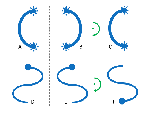
A great simplification to the general VRTE (Eq. 2 of the previous page) results if the scattering particles are assumed to be (1) randomly oriented and (2) “mirror symmetric.” The concept of mirror (or bilateral) symmetry is illustrated in Fig. 1. Panel A represents a particle. The dashed line represents a mirror, and particle B is the mirror image of A. This B does not “look like” or overlay A. However, if B is rotated by 180 deg about an axis normal to the plane of the figure, as illustrated by the green arrow, B becomes C, which looks exactly like A (is congruent with A). This means that A is a mirror-symmetric particle. Particle D has mirror image E. Rotating D by 180 deg about a vertical axis gives F, which (even without the “head”) cannot be made to overlay D. This means that the shape of D is not mirror symmetric. In general, a particle is mirror symmetric if a translation and/or rotation of the mirror-reflected particle can make it congruent with the original particle.
Suppose that the scattering medium consists of randomly oriented, mirror-symmetric particles. The bulk medium is then directionally isotropic and mirror symmetric. In this case, the extinction matrix becomes diagonal, with each element equal to . There is thus a common extinction coefficient for all states of polarization and directions of propagation:
| (1) |
Here is the oceanographers’ “beam attenuation coefficient.” (In Mishchenko’s notation, , which explicitly shows the contributions of the background medium (the water; the term) and the imbedded particles.)
In addition, the scattering matrix becomes block diagonal and the scattering depends only on the included angle between directions and , and not on the directions and themselves. This scattering angle is given by
The form of the scattering matrix is then (Mishchenko et al. (2002))
| (2) |
The restriction to an isotropic, mirror-symmetric medium gives a scattering matrix with only six independent elements.
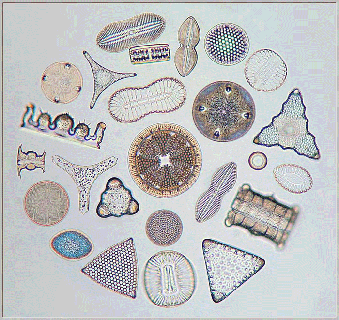
The obvious question is now, “How realistic is the assumption that oceanic particles are mirror-symmetric?” Figure 2 shows a collection of oceanic diatoms (arranged for artistic purposes). Many of these are clearly not spherical (contrary to what is often assumed by modelers who can’t wean themselves away from Mie theory), but they all appear to be mirror-symmetric to a good approximation. The same holds true for many other species of phytoplankton which, if not roughly spherical, at least have bilateral symmetry. Likewise, atmospheric particles such as fog droplets, snowflakes, and ice crystals are often mirror symmetric. Use of Eqs. (1) and (2) is then justified.
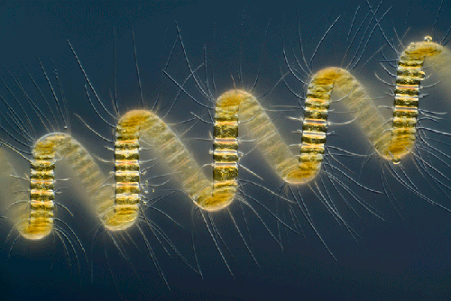
Of course, this is not always the case. Figure 3 shows a photo of a chain-forming diatom Chaetoceros debilis. This cute little fellow appears to be a left-handed helix (assuming that the original image has not been flipped). Chiral (left- or right-handed) particles are not mirror symmetric. If the ocean contains lots of such particles (e.g., during a bloom), and all have the same handedness, then you have solve Eq. (2) of the previous page (perhaps with the simplification to one spatial dimension). Of course, no one ever does that, which is one more reason that numerical predictions of radiances may not agree perfectly with measurements. However, if there are equal numbers of randomly oriented left- and right-handed helical particles, then the bulk medium itself is mirror symmetric even though the individual particles are not, and the simplified VRTE is still applicable.
Consider next the calcium carbonate plates that are at times shed by cocolithophores. The material itself, , is birefrengent (meaning that the real index of refraction depends on the polarization), so in general would require the full 16-element matrix to describe the polarization-dependent extinction. However, the shapes of the liths (little platelets of ) are mirror symmetric. So if the water is filled with randomly oriented liths, and the spatial distribution of the refractive index is also randomly oriented, then the bulk medium is mirror symmetric and Eqs. (1) and (2) are applicable. Likewise, the medium might contain spherical beads of dichroic glass (dichroic means that the imaginary index of refraction depends on the polarization). The spherical shape is mirror symmetric. However, if the spatial pattern of the dichroism is not random, then the full VRTE must be used. If the beads are randomly oriented in the pattern of dichroism, then the bulk medium is again mirror symmetric and Eqs. (1) and (2) are applicable.
There are very few measurements of scattering matrices for ocean waters. However, those that have been made indicate that the form of seen in Eq. (2) is a reasonable approximation. The reduced scattering matrix is defined as the scattering matrix with each element normalized by the element, which is the volume scattering function for scattering of unpolarized light into unpolarized light. That is, .
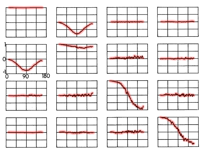
Figure 4 shows measurements of the reduced scattering matrix for a location in the Atlantic Ocean. To a good approximation, the matrix elements shown in this figure obey the symmetries shown in Eq. (2). The measured is block symmetric with and (although both of those elements are zero to within a bit of noise). In addition, , which is characteristic of rotationally symmetric particles. For spherical particles, in addition, ; these are noticeably, but not greatly, different in the measured matrix elements. Similar results were obtained for about 200 measurements in Atlantic, Pacific, and Gulf of Mexico waters. Thus observation supports the use of scattering matrices of the form of Eq. (2), corresponding to the assumption of non-spherical but mirror-symmetric particles, except for unusual circumstances such as a bloom of helical phytoplankton like those of Fig. 3.
In summary, the assumption of randomly oriented, mirror-symmetric particles gives an isotropic, mirror-symmetric medium with two very important simplifications to the general VRTE: (1) the attenuation coefficient does not depend on direction or state of polarization, and (2) the scattering matrix has only six independent elements, which depend only on the scattering angle (and of course on location and wavelength). Figure 2 should convince you that the additional assumption of an ocean dominated by spherical phytoplankton may not be valid except during bloom conditions by a species that is nearly spherical.
If we further assume that the optical properties of the ocean depend only on depth , and that the boundary conditions are horizontally homogeneous, then the left hand side of the three-dimensional VRTE reduces to a one-dimensional, ordinary (in space) derivative,
Likewise, the other location arguments simplify to depth only. The resulting one-dimensional (1D) VRTE then reads
Here has the form shown in Eq. (2) and the rotation matrices have the form seen in Eq. (3) of the previous page. In polar coordinates, the element of solid angle is given by . The integration is over all steradians of the incident directions.
Equation (3) along with Eq. (2) is as far as we should go in simplifying the VRTE if we are interested in computing underwater polarized radiance distributions.
To solve Eq. (3) requires knowledge of the , and elements of the phase matrix. Several modern instruments have been developed for in situ measurement of the VSF, , over a wide range of scattering angles (e.g., Lee and Lewis (2003), Harmel et al. (2016), Li et al. (2012), Tan et al. (2013)). The POLVSM instrument described in Chami et al. (2014) can measure the nine elements of that do not involve circular polarization, i.e. . The MASCOT instrument of Twardowski et al. (2012) measures the top row of , i.e. . The LISST-VSF, Slade et al. (2013), measures and . Only the LISST-VSF is commercially available. Not even the VSF is routinely measured during oceanographic field work. Therefore, when the VRTE is solved, usually some model is used to create the needed scattering matrix elements. This model is often Mie theory, which assumes spherical particles.
The three-dimensional VRTE is most commonly solved by Monte Carlo techniques. The assumption of a one-dimensional geometry gives a VRTE that is amenable to a variety of other numerical solution techniques, which have been employed in many studies of atmospheric and oceanic light fields.
 See comments posted for this page and leave your own.