Page updated:
October 14, 2021
Author: Curtis Mobley
View PDF
Anomalous Dispersion
When the real index of refraction decreases with increasing wavelength (i.e., , or ) the associated dispersion is called “normal” dispersion. This is the situation for water or glass at visible wavelengths. According to Snell’s law, red light will deviate less than blue when passing from air into a water drop. The result is that the red band of color (longer wavelengths) is at the outside of a rainbow, and the violet (shorter wavelengths) is at the inside. Regions of the spectrum where increases with wavelength (, or ) would give the reverse order of wavelengths: shorter wavelengths would be at the outside of the rainbow and longer wavelengths at the inside. This reversal of “colors” from that seen in normal life at visible wavelengths is called “anomalous dispersion.” There is really nothing normal or abnormal about either situation, you simply get a particular order of refracted wavelengths depending on the sign of .
Anomalous dispersion occurs near strong absorption bands, which is how it enters into the understanding of the optical properties of phytoplankton, e.g. in papers by Morel and Bricaud (1981), Morel and Bricaud (1981b), Bricaud et al. (1983), Bricaud and Morel (1986), and Stramski et al. (1986). Because of this important application, anomalous dispersion warrants discussion. To understand anomalous dispersion, we must construct a model for light propagation in a dielectric. A simple, but very fruitful and still useful, model was constructed by H. A. Lorentz around 1900. [This is the same Lorentz of the Lorentz transformation in special relativity and of many other results that still bear his name. He shared the 1902 Nobel Prize with Zeeman for their discovery and explanation of the Zeeman effect, which is the splitting of some spectral lines in the presence of a magnetic field. His model of light propagation in dielectrics grew out of his efforts to understand the physical basis for the index of refraction. His work was one of the first couplings of Maxwell’s equations with the new “electron theory of matter” after the discovery of the electron in 1897.] I will merely outline the development of the Lorentz model—the details are a standard topic in texts on classical electrodynamics; see, for example, Section 8.4.2 of Griffiths (1981). The arguments are as follows.
Electrons in a dielectric are bound to specific molecules by electrostatic forces from the nuclei. When an electromagnetic wave of frequency passes by, the oscillating electric field causes the electrons to oscillate at the same frequency as the wave. However, the electrons also have resonant or “natural” frequencies . If the incident wave frequency is near to resonate frequency, the light-molecule interaction is particularly strong.
Let be the displacement of an electron of charge and mass from its equilibrium position in the molecule. When the electron is pulled away from its equilibrium position at there is a binding or restoring force that pulls it back towards its equilibrium position:
If the sign of the force pulling the electron away from equilibrium is taken to be the positive direction, then the binding force pulling it back is in the negative direction. If the electron is set in motion by a passing electromagnetic wave, it will oscillate forever unless there is some damping force. That force is taken to be proportional to the speed of the oscillating electron:
where is a measure of the strength of the damping. The nature of the damping need not concern us here, but one mechanism is “radiation damping,” which arises because oscillating (i.e., accelerated) charges radiate energy. The driving force is the electromagnetic field:
The total force on the electron is then
which gives the equation
This is the equation for a damped harmonic oscillator. Thus the electrons are modeled in classical physics terms as though they are charged masses tied to molecules like a masses on springs driven by an applied sinusoidal force. This equation is linear, so we can replace the terms with complex representations, just as was done in the previous pages on wave propagation:
In steady state conditions, the electron oscillates at the driving frequency:
Inserting this into the previous equation gives
The dipole moment induced by the electric field is the product of the charge and the distance from equilibrium:
If is the number of electrons per cubic meter in the material, then the bulk polarization is . Moreover, there are many electrons in a molecule, each of which has its own resonant frequency, denoted for the electron. Each electron contributes to the bulk polarization, so we sum over all electrons to obtain
where is the number of electrons in each molecule with resonant frequency and damping parameter .
Now recall from the previous page that the polarization vector was written as . We now introduce a complex susceptibility and write the magnitudes as . Recall also that the proportionality between the the displacement field and the electric field is , so we now introduce a complex permittivity . Assembling these pieces gives the Lorentz model for the permittivity:
| (1) |
We also recall from Eq. (15) of the plane waves page that the complex wave number was written as
where is the complex index of refraction.
To simplify the math, let us assume that the term is small compared to 1, and that , so that we can write
We now have
| (2) |
The summands in this equation are complex numbers of the form , which can be written as
This make it easy to extract the real and imaginary parts of Eq. (2). Recalling that the real index of refraction is and that the absorption coefficient is gives
| (3) |
and
| (4) |
Equation (3) is what Lorentz was after: a model linking parameters of the substance, e.g., the density of electrons and their resonant frequencies, to the index of refraction. His development also gave a model for the absorption coefficient with no additional effort. The shape of the absorption curve defined by Eq. (4) is called a Lorentzian line shape. (There are other line shapes that describe effects in gases such as pressure broadening and Doppler shifting, but these do not concern oceanographers.)
The limiting cases of the Lorentz model are worth noting. At very low frequencies (), the permittivity seen in Eq. (1) becomes real and of the form , where is now a constant that depends on the particular substance. Water is a highly polar molecule, which means that the bulk polarization achieves a large magnitude as the water molecules align themselves with the slowly varying electric field. This gives a large value for and thus for . For water, at low frequencies. This gives a real index of refraction , which is seen in Fig. (1) of the water IOPs page for (). For very high frequencies, , the term in the denominator of Eq. (1) dominates because the applied frequency is greater than any resonant frequency of the molecule. The permittivity then has the form . Thus the index of refraction approaches 1 from values less than 1 as . This is true for any substance, and is seen for water in Fig. (1) of the water IOPs page or Fig. 4 of the Dispersion page for ().
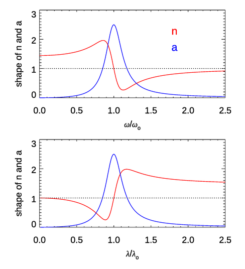
Figure 1 shows the shapes of the functions for the index of refraction and the absorption coefficient near a single resonant frequency. (That is to say, the plot shows the frequency-dependent function without the factor and similarly for the plot. A value of was used.) For most of the frequency range, (or ). This is the case of “normal” dispersion. However, near the absorption line, the derivative of is reversed. This is the case of “anomalous dispersion.” In materials like water there are many absorption lines due to electronic transitions (in the UV), vibrational modes (in the near IR), and rotational modes (in the far IR and longer wavelengths). These lines are often closely spaced, so they tend to overlap and blur out the features seen here for a single isolated line, and can remain above 1. However, near very strong absorption features, the anomalous dispersion effect on the index of refraction can be seen. This is the case near and in Fig. 4 of the Dispersion page, where the shape of the curve looks qualitatively like that of the bottom panel of Fig. 1. These features are due to strong vibrational modes of the water molecule (O-H stretching modes). The structure of in at wavelengths from 0.115 to is due to a number of electronic transitions. Note also that as the frequency increases (the wavelength decreases), approaches 1 from values less than 1. This is the behavior seen in Fig. 4 of the Dispersion page.
To finish the discussion of the Lorentz model, it is first noted that the assumption that was small compared to 1 is fairly good for gases. However, for liquids and solids, where one molecule interacts with its neighbors and not just with the sinusoidal electric field, the equations seen here require modification to allow for the “packing” of the molecules in space. That leads to a result known as the Clausius-Mosotti, or the Lorentz-Lorenz, equation. However, that modification does not change the basic idea developed here and need not be pursued. Of course, real electrons are not attached to molecules as though they were on springs. Somewhat surprisingly, a proper quantum mechanical treatment of the problem leads to a result with exactly the same functional form as seen in Eq. (1). However, the various terms are interpreted differently. The resonant frequencies are replaced by the frequencies corresponding to the energy differences between the quantized energy levels in the atom or molecule, and so on.
Kramers-Kronig Relations
At first glance it would seem that the real index of refraction and the absorption coefficient should be unrelated optical properties of a material. As emphasized on the Physics of Scattering page, spatial changes in the index are responsible for scattering. Absorption, on the other hand, describes how energy is removed from a beam of light. However, as seen in the development of the Lorentz model, equations for both the index of refraction and the absorption coefficient were obtained from the same analysis of how matter responds to a sinusoidal electromagnetic wave, i.e. to light. The frequency-dependent functions for and are very similar in form. This hints at a deeper connection between and .
There is indeed a profound connection between the real index of refraction and the absorption coefficient. These two quantities are in fact so closely related that if you know one at all wavelengths, you can compute the other at all wavelengths. This relation was discovered independently by R. de L. Kronig in 1926 and by H. A. Kramers in 1927. The derivation of these equations is mathematically difficult and will not be give here; see Section 2.3.2 of Bohren and Huffman (1983) for a discussion.
Kramers-Kronig equations relate the real and imaginary parts of what are called analytic functions. Without going into the details, there are many physical functions that satisfy the requirements to be analytic. Examples relevant to optics are the frequency dependent complex index of refraction and related quantities such as the complex dielectric function and the electric susceptibility . When stated for the complex index of refraction , the Kramers-Kronig relations are (Eqs. 2.49 and 2.50 of Bohren and Huffman (1983))
If these equations do not scare you, they should. Note that as the frequency is integrated from 0 to , somewhere along the way the integration variable will equal and the denominator of the integrand will equal 0, while the numerator is non-zero. Thus the integrand becomes infinite and the integral diverges. The symbol in front of the integrals indicates the Cauchy principle value of the integrals. The Cauchy principle value is a way to assign a finite value to some divergent integrals by computing a contour integral in the complex plane, “going around” the singular point, and then taking suitable limits. [To learn how that is done, you need to take a class in complex analysis, where you will learn about wonderful things like poles, residues, branch points, contour integration of complex functions and, of course, how to evaluate Cauchy principle value integrals. The standard text on this topic was published by R. V. Churchill in 1948. It is still in press as an edition Brown and Churchill (2009).] The mathematical details are not needed for the present discussion, which will take as given that the integrals can be evaluated.
The absorption coefficient is determined by the imaginary part of the index of refraction via Eq. (20) of the plane waves page: . Using this and the relation allows the previous form of the Kramers-Kronig relations to be converted into the corresponding form for and :
These equations are not just of academic interest. For example, it is often easier to measure the absorption coefficient than the index of refraction. Then a measurement of absorption allows the determination of the index of refraction via Eq. (7). This is what Zoloratev and Demin (1977) did, although they do not give the details of their numerical calculations. Segelstein (1981) did essentially the same thing, although he did his numerical calculations using a fast Fourier transform technique derived from the Kramers-Kronig relation (5).
It is important to note that you cannot measure absorption at one frequency (or wavelength) and then determine the index of refraction at that frequency. You have to measure over all frequencies, and then you can determine over all frequencies by repeated evaluations of Eq. (7). In practice you never have measurements over all frequencies, but you have to have measurements over a wide-enough range of frequencies to enable an accurate approximate evaluation of the integrals. Of course, the integrations must be performed numerically, which is not trivial because of the singularity at . There is considerable literature on this; Fitzgerald (2020) gives a listing of Matlab code to carry out the calculations.
The purpose of this brief discussion of Kramer-Kronig relations is to show that absorption and the real index of refraction are closely related. You might have a need for a material with particular absorption and refractive properties. So you mix together just the right combination of dyes to give the absorption spectrum you want. However, at that point you have no freedom to someway define the real index of refraction; it has now been fixed by Eq. (7).
There is much more to be said about Kramers-Kronig relations, which occur throughout physics and engineering. They are much more general than just the forms seen here for optical variables. At the deepest level, they are a necessary and sufficient for causality, which means that an effect cannot occur before its cause. This also means that no signal can propagate faster than the speed of light in a vacuum. A necessary and sufficient condition that a signal speed in a medium be less than the speed of light is that the real and imaginary parts of the medium’s refractive index satisfy Eqs. (5) and (6).
 See comments posted for this page and leave your own.