Page updated:
October 13, 2021
Author: Curtis Mobley
View PDF
The General Vector Radiative Transfer Equation
The goal of this page and the next two is to obtain the vector and scalar radiative transfer equations in the forms that are commonly used in optical oceanography. The steps to these equations are outlined starting from the most fundamental physics. This sequence makes explicit what assumptions must be made along the way to get from an exact but highly abstract and mathematical theory to equations that are only approximate but which can be solved to get results that are accurate enough for many applications. In particular, the presentation shows what is given up at each step in exchange for increased simplicity in the resulting physics and mathematics. The final result will be the scalar radiative transfer equation (SRTE), which is seen in many textbooks and which is solved by the widely used HydroLight radiative transfer software.
The phenomenological nature radiative transfer theory as developed over the decades made its connections to fundamental physics unclear because of its heuristic derivations and (sometimes physically indefensible) assumptions (e.g., Preisendorfer (1965), Mishchenko (2013), and Mishchenko (2014)). Theoreticians worked for decades to construct ”an analytical bridge between the mainland of physics and the island of radiative transfer theory”, as R. W. Preisendorfer worded it (Preisendorfer (1965), page 389). Most recently, M. I. Mishchenko has expended enormous effort to develop a physically and mathematically rigorous connection between Maxwell’s equations and the vector radiative transfer equation (VRTE), from which the SRTE is obtained after further simplifications. Thus Preisendorfer’s bridge has now been completed with a level of rigor worthy of any branch of physics (e.g., Mishchenko (2008a), Mishchenko et al. (2016)). This page outlines how that bridge is constructed.
The path from fundamental physics to radiative transfer theory works it way through the following stages:
- 1.
- Quantum Electrodynamics
- 2.
- Maxwell’s Equations
- 3.
- The general vector radiative transfer equation (VRTE)
- 4.
- The VRTE for particles with mirror symmetry
- 5.
- The SRTE for the first component of the Stokes vector
Notation: This and the following pages use bold face and for electric and magnetic field vectors, and for the current vector, in 3-D space. Stokes vectors and matrices are denoted by “blackboard” fonts: , etc.
Quantum Electrodynamics
Quantum electrodynamics (QED) is the fundamental physical theory that explains with (as far as we know) total accuracy the interactions of light and matter, or of electrically charged particles. In this theory, the electromagnetic field itself is quantized, and the photon is the quantum of the field. The electromagnetic force between charged particles is described by the exchange of so-called virtual photons (called ”virtual” because they are not detectable in the roll of transferring forces between charged particles). The photon is said to mediate or carry the electromagnetic force.
As an example of the accuracy of QED, the most recently measured value of a quantity called the electron spin g-factor is (Hanneke et al., 2011. Phys. Rev. A DOI: 10.1103/PhysRevA.83.052122)
where the last two digits in parentheses give the uncertainty in the preceding two digits. The value predicted by the most recent QED calculations is (Aoyama et al., 2015. Phys. Rev. D DOI: 10.1103/PhysRevD.91.033006)
This is an agreement between theory and experiment of around 1 part in , which is an accuracy equivalent to measuring the circumference of the Earth to within 0.04 millimeters. Similar results are obtained for other QED predictions. Because of its exceptional success in explaining nature at its most fundamental level of elementary particle interactions, QED is often regarded as the most successful theory in physics.
Unfortunately, QED is exceptionally abstract and mathematical, and the calculations can be carried out only for simple interactions, such as the scattering of one elementary charged particle by another (although the calculations for even the simplest of interactions can be exceedingly complex according to the rules of QED). QED is the conceptual starting point for much of modern physics, but it isn’t even remotely practical for everyday calculations. If you want to start learning about how the theory is formulated, there is no better place to begin than Feynman’s classic popular exposition QED: The Strange Story of Light and Matter. After that, if you want to get a bit more serious and see how the calculations are actually done, the best text I’ve found is Introduction to Elementary Particles, Second Edition by Griffiths. Learning about QED a fascinating journey, but this is not a road that oceanographers are required to travel.
Maxwell’s Equations
QED is a quantum field theory that describes light and electromagnetism at the level of individual photons, which in QED are viewed as the quantized vibrational modes of the electromagnetic field. It is possible to take a “classical physics limit” of QED to get a classical field theory, in which the electromagnetic field is not quantized. The result is Maxwell’s equations, which describe electric and magnetic fields as continuous functions of space and time. One way to think of this limiting process was stated by Sakurai (1967) as “The classical limit of the quantum theory of radiation is achieved when the number of photons becomes so large that the occupation number may as well be regarded as a continuous variable. The space-time development of the classical electromagnetic wave approximates the dynamical behavior of trillions of photons.” Not surprisingly, getting from QED to Maxwell requires a high level of mathematical and physical sophistication.
Maxwell’s equations for the electric field (units of ) and magnetic field () at location and time are (in differential form, in SI units)
Here is the electric charge density () and is the electrical current density () in the region of interest. The quantity is the electric permittivity of free space, and is the magnetic permeability of free space; these are fundamental physical constants.
These equations are applicable to the every-day needs of science and engineering. They govern matters as seemingly diverse as the generation, propagation, and detection of radio waves; the generation of electrical power for your house; the generation of Earth’s magnetic field, the refraction of light at an air-water surface, and the scattering of light by phytoplankton. However, the greatest achievement of Maxwell and his equations is this: In “free space,” i.e. when and , a bit of vector calculus shows that each of the , , and components of the and vectors satisfies an equation of the form
This equation describes a wave propagating with speed . Plugging in the numbers for and gives . As Maxwell observed in 1862, “This velocity is so nearly that of light that it seems we have strong reason to conclude that light itself (including radiant heat and other radiations) is an electromagnetic disturbance in the form of waves propagated through the electromagnetic field according to electromagnetic laws.” This result is one of the greatest intellectual achievements of all time: not only were electric and magnetic fields tied together in the first unified field theory in physics, but light was shown to be an electromagnetic phenomenon.
The and wave solutions coming out of Maxwell’s equations contain full information about the phases of the fields. Maxwell’s equations can thus describe interference phenomena, which depend on the instantaneous phases of the fields.
Maxwell’s equations are discussed in more detail beginning on page Maxwell’s Equations in Vacuo.
Although Maxwell’s equations are very accurate for predicting the phenomena of classical physics, they do fail when applied to atomic-scale processes, extremely strong fields, and the realm of “quantum optics,” which deals with individual photons. In particular, classical physics failed to describe blackbody radiation and the photoelectric effect, which is why Planck and Einstein had to make radical new assumptions in order to explain the observations. Those assumptions were the start of quantum mechanics. (To be precise, benefitting from the insights of a century of quantum mechanics, the failure of classical physics to describe the photoelectric effect and blackbody radiation was not due to the radiation field not being quantized (Maxwell’s equations), but due to the discrete nature of atomic absorption and emission processes, which in turn lead to discrete harmonics of the associated radiation. But that’s another story....)
For solution in material media, Maxwell’s equations must be augmented with information about the electrical and magnetic properties of the material and with boundary conditions describing the specific problem of interest, such as sunlight passing through the sea surface and propagating through an ocean full of absorbing and scattering particles. (The equations do become somewhat more complicated in material media, although the general form remains the same.) These equations do find occasional use in oceanography. For example, they have been for measurement of ocean currents via the electric fields set up by a conductor (salt water) moving through the earth’s magnetic field (e.g., Larsen (1973), Larsen (1992)). They are also the foundation for computations of sea ice emissivity and reflection at microwave frequencies (e.g., Tan et al. (2016)). However, those applications are either non-optical or at wavelengths far longer than the visible spectrum. Direct numerical solutions of Maxwell’s equations are reviewed in Section 7 of Mishchenko et al. (2016).
For geometry as complex as a wind-blown sea surface and a water column filled with spatially varying absorbing and scattering matter, Maxwell’s equations and their boundary conditions are just too complex to solve for typical optical oceanographic problems. So, elegant and useful as they are for some problems, optical oceanographers must seek still further simplifications.
The General Vector Radiative Transfer Equation
The next simplifying step is to go from the world of electric and magnetic fields to the world of radiance. At optical wavelengths, the frequency of electromagnetic waves (light) is of order Hz. This is far higher than can be directly measured for a time-dependent propagating field. In practice, time-averaged irradiances are measured, in conjunction with various combinations of polarizing filters, over times long compared to the wave period. This time-averaging destroys the phase information contained in the instantaneous vector fields, but preserves the directional information about the plane of oscillation of the (and ) field, i.e., it preserves information about the state of polarization of the light.
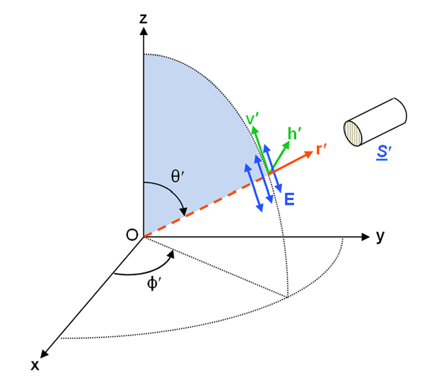
As described on the Polarization: Stokes Vectors page, the state of polarization of a light field is specified by the four-component Stokes vector, whose elements are related to the complex amplitudes of the electric field vector resolved into directions that are parallel () and perpendicular () to a conveniently chosen reference plane. In the oceanographic setting, this reference plane is usually the meridian plane, which is defined by the normal to the mean sea surface, , and the azimuthal direction of the propagating light; the meridian plane is thus perpendicular to the mean sea surface. In a polar coordinate system , is the polar angle component of the electric field and is the azimuthal angle component. Figure 1 shows the meridian plane as commonly used for oceanography radiative transfer calculations.
There are two versions of the Stokes vector seen in the literature, and these two versions have different units and refer to different physical quantities. The coherent Stokes vector describes a quasi-monochromatic plane wave propagating in one exact direction, and the vector components have units of power per unit area (i.e., irradiance) on a surface perpendicular to the direction of propagation. For a propagating electric field of the form (see Plane Wave Solutions), where the wavenumber vector is in the direction of propagation, and with the choice of the meridian plane as the reference, the coherent Stokes vector is then defined as (Mishchenko et al. (2002))
| (1) |
Here is the electric permittivity of the medium (SI units of ), and is the magnetic permeability of the medium (). Thus the elements of the coherent Stokes vector have units of or , i.e. of irradiance. denotes complex conjugate, hence the components of the Stokes vector are real numbers. Note that the values of the and elements of the Stokes vector depend on the choice of reference plane, whereas and do not.
The diffuse Stokes vector is defined as in Eq. (1) but describes light propagating in a small set of directions surrounding a particular direction and has units of power per unit area per unit solid angle (i.e., radiance). It is the diffuse Stokes vector that appears in the radiative transfer equations as developed here. The differences in coherent and diffuse Stokes vectors are rigorously presented in Mishchenko et al. (2002).
Authors often omit the factor in Eq. (1) because they are interested only in relative values such as the degree of polarization, not absolute magnitudes, but this omission is both confusing and physically incorrect. Units and magnitudes matter! In particular, the different units of coherent and diffuse Stokes vectors, and whether or not the factor is included in the definition of the Stokes vector, have subtle but very important consequences regarding how light propagation across a dielectric interface such as the air-water surface is formulated (e.g., Garcia (2012), Zhai et al. (2012)).
The transition from electric and magnetic fields to Stokes vectors yields a general 3D vector radiative transfer equation. Let denote the Stokes vector at spatial location for light propagating in the direction: . Then the VRTE has the form (Mishchenko (2008a), with slightly different notation and with the addition of an internal source term)
| (2) |
In this equation,
- is a extinction matrix, which describes the attenuation (by the background medium and any particles imbedded in the medium) of the light propagating in direction .
- is a phase matrix, which describes how light in an initial state of polarization and direction in the incident meridian plane is scattered to a different state of polarization and direction in the final meridian plane.
- is a internal source term, which specifies the Stokes vector of any emitted light such as bioluminescence or light at the wavelength of interest that comes from other wavelengths via inelastic scattering.
In general, all 16 elements of and are nonzero, and they depend on both location and direction (and wavelength; not shown). Equation (2) can describe polarized light propagation in matter that is directionally non-isotropic (e.g., in a crystal), that can absorb light differently for different states of polarization (linear or circular dichroism), and that contains scattering particles of any shape and random or non-random orientation. (See Mishchenko et al. (2002) or Mishchenko et al. (2016) for a rigorous discussion of how these matrix elements are defined and computed. The of Eq. 2 is a bulk extinction matrix. In Mishchenko’s papers this is written as , where is the number of particles in the volume of interest , and is a single-particle extinction matrix averaged over all particles. A similar comment holds for .)
By definition the phase phase matrix scatters light from one meridian plane (defined by and ) to another (defined by and ). It is customary to write as a product of three matrices that
- 1.
- Transform the initial (unscattered) Stokes vector from the incident meridian plane to the scattering plane, which is the plane containing the incident () and scattered () directions,
- 2.
- Scatter the Stokes vector from direction to , with calculations performed in the scattering plane, and
- 3.
- Transform the final Stokes vector from the scattering plane to the final meridian plane.
When this is done, the phase matrix is written as
| (3) |
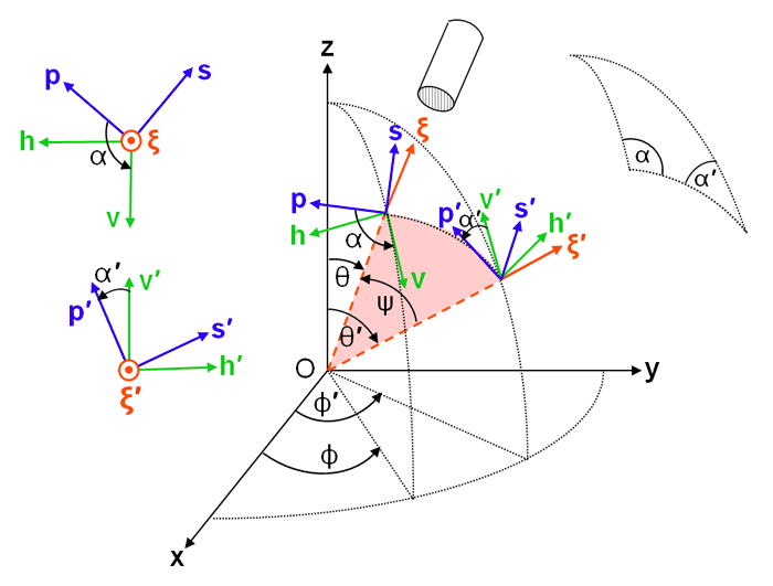
Here is a matrix that transforms (“rotates” through an angle ) the incident Stokes vector into the scattering plane; is a matrix, the scattering matrix, which by definition scatters the incident Stokes vector to the final Stokes vector, with both expressed in the scattering plane; and is a matrix that rotates the final Stokes vector from the scattering plane to the final meridian plane. (In general, is called the scattering matrix. In the laboratory setting, is usually called the Mueller matrix.) This factoring of separates the physics of the scattering process () from the geometrical bookkeeping related to the coordinate systems (the rotation matrices). For the choice of a positive rotation being counterclockwise when looking into the beam, the Stokes vector rotation matrix is (e.g., page 25 of Mishchenko et al. (2002))
| (4) |
The rotation angles and are shown in Fig. 2 These angles determined by spherical trigonometry as described on the Polarization: Scattering Geometry page.
Equation (2) is almost never applied to oceanic problems. The reason is less for mathematical reasons than because there are no comprehensive data or models for the needed inputs and . To be useful, all elements of these matrices must be available for a wide range of oceanic waters. Further simplification is required.
 See comments posted for this page and leave your own.