Page updated:
October 13, 2021
Author: Curtis Mobley
View PDF
Plane Wave Solutions
Now that we have been introduced to Maxwell’s Equations on the previous two pages, we can attempt to solve them. Textbooks on classical electrodynamics (e.g., Jackson (1962), Griffiths (1981), Bohren and Huffman (1983)) take a general approach of assuming little and letting Maxwell’s equations force upon you conclusions about what functional forms of solutions are possible for propagating waves. This is not a physics text, so I will propose a form for propagating electric and magnetic fields and show that they satisfy Maxwell’s equations. That approach is sufficient to show with a minimum of math and physics how waves can propagate in dielectrics like water. In so doing, we will discover the relation between the absorption coefficient and the imaginary parts of the index of refraction and the wave number. The discussion of plane waves on this page sets the stage for a deeper investigation of wave propagation on the next two pages, which are on dispersion.
Plane Waves in a Dielectric
Other than electromagnetic waves propagating in a vacuum, the simplest solution of Maxwell’s equations for wave propagation is for a plane wave in a dielectric material. The term “plane wave” refers to an electromagnetic wave (i.e., light) that is propagating in some direction, and which has the same properties at all points of a plane perpendicular to the direction of propagation. As will be seen, if we know the electric field of the wave, we can find the magnetic field from Maxwell’s equations (or vice versa). Thus it is customary to consider only the electric field of the wave.
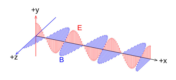
Consider first an electromagnetic wave propagating in a vacuum. We are free to choose a convenient coordinate system, so let the wave propagate in the direction, and let the electric field oscillate in the direction (i.e., the electric field is linearly polarized in the direction). The associated magnetic field then oscillates in the direction. This situation is illustrated in Fig. 1.
We can write the magnitude of the electric field as
| (1) |
where sets the magnitude of the electric field, is the angular wave number, and is the angular frequency; is the wavelength and is the period of the oscillation. For propagation in a vacuum, ; i.e., a wave propagating at the speed of light travels a distance in one period of the oscillation. It is common to use rather than for the wavenumber; the reason for my choice of will be explained below.
Electric fields, wave numbers, frequencies, and the like are of course real quantities. However, it will prove to be convenient to write the electric field of Eq. (1) as the real part of a complex quantity:
where stands for the real part of the argument, and we recall that where . Some authors use a subscript c to indicate a complex field, and some use a tilde, and some leave it to the reader to figure out from the context which variables are real and which are complex. I will use a tilde and write
In the second equation, the phase angle has been incorporated into the amplitude so that . Now , and so on. It is customary to omit writing the symbol, in which case it is understood that at the end of any calculation involving complex numbers we must take the real part to get back to a real physical quantity. Some authors call the “complex electric field”, but a better terminology is to say that is the complex representation of the real electric field .
We can rewrite (2) as
It is easily shown by substitution that any function of the form , where is a constant scale factor, satisfies the 1D wave equation
Thus any function of the form describes a function with shape at time propagating in the direction with speed . We can thus identify the speed
| (3) |
as the speed of the electromagnetic wave. This speed is known as the phase speed of the sinusoidal wave because it shows how fast a point with a given phase of the sinusoidal wave, say the wave crest, travels.
A function of the form propagates with an amplitude that is independent of time and location. That is correct for propagation in a vacuum. However, in absorbing matter, the Bouguer-Lambert-Beer law says that the irradiance attenuates exponentially with distance according to , where is the absorption coefficient. We can build this attenuation into the electric field in an ad hoc manner by replacing the constant amplitude of the electric field with a function of with the form
where is a positive constant. (The means “is replaced by”.) Equation (2) is then replaced by
Here is called the complex wave number. I will omit writing since there is no ambiguity with another usage for .
Before proceeding, we must face a problem of notation. On the water IOPs page, I wrote the complex index of refraction as , where was the real index of refraction and was called the imaginary part of the index of refraction. It is also common to use as the wavenumber: . Every author seems to have a slightly different way to avoid using the same symbol for two different quantities. Bohren and Huffman (1983) use a Roman for the complex wavenumber, which they write as , and they use an italic for the imaginary part of the index of refraction. They also use rather than for the complex index of refraction. Thus my is Bohren and Huffman’s . Griffiths (1981) uses for the real part of the complex wavenumber and for the complex part. Thus he writes the complex wavenumber as . Mishchenko et al. (2002) write and . For this page and the next, I have chosen to use for the imaginary part of the index of refraction and for the wavenumber, with a single prime on the real part and a double prime on the imaginary part. You will similarly see the complex index of refraction written as . To further complicate matters, some authors write the time dependence in Eq. (1) as , in which case the complex index of refraction (in my notation) becomes and the complex wavenumber is . The whole notation business is a mess, and you just have to figure out each author’s preferences.
Now let us turn the electric and magnetic fields into vectors so we can insert them into Maxwell’s equations. In Fig. 1 the electric field oscillates in the plane, and the magnetic field lies in the plane. So for these fields we can write
At this point I have proposed two traveling waves for the electric and magnetic fields. Now we can ask, “under what conditions do waves of the form of Eqs. (5) and (6) satisfy Maxwell’s equations?”
Recall that Maxwell’s equations in matter are
with the constitutive relations
For a linear medium, is proportional to and is commonly written , where is the electric susceptibility (i.e., measures how susceptible the material is to being polarized by an electric field). is assumed to be independent of and is independent of location and direction in a homogeneous, isotropic medium. Thus . The quantity is the permittivity of the medium. If we assume that there are no free electric charges in the medium (), the first of Maxwell’s equations (Eq. 7) is . Inserting the complex representation into gives
after noting that and that the and derivatives are 0 because the wave varies only in . Thus the form of Eq. (5) for satisfies . Likewise, the form of Eq. (6) for satisfies .
Next insert the proposed and into Eq. (9). The result is
This equation is satisfied only if
| (13) |
Thus, given the electric field, we can compute the magnetic field. Taking the real parts of this equation gives
| (14) |
after recalling the definition of the phase speed from Eq. (3), and recalling that the speed of light in a medium with real index of refraction is the speed in vacuo divided by .
For a dielectric, the magnetization is zero, so , where is the permeability of the medium. (In general one can write , where is the magnetic susceptibility of the medium. In a dielectric, is very nearly equal to , the permeability of a vacuum.) If there are no free currents (), the remaining Maxwell equation 10 reduces to
Inserting the complex representations into this equation gives
or
This result combined with that of Eq. (13) implies that
or
When the wave equation is derived starting with Maxwell’s equations in matter, the wave speed is (rather than as was seen in Eq. (10) of the previous page for the vacuum case). The speed of light in a medium with real index of refraction is . Given that in the last equation is complex (which implies that and/or must also be complex, as will be seen in the discussion of dispersion), we can introduce the complex index of refraction and write
| (15) |
after recalling that is the free-space wavenumber .
We can now rewrite the complex representation of the electric field as
Taking the real part gets us back to the real electric field:
| (18) |
The corresponding equation for is
| (19) |
or an equivalent based on Eq. (14).
We have now shown that sinusoidal plane waves can propagate through a dielectric provided that the magnitude of the magnetic field is proportional to the magnitude of the electric field according to Eq. (14), and that the wave number is related to the angular frequency according to Eq. (15).
The Absorption Coefficient
The equations above are for electric and magnetic fields, which are what physicists like to play with. Oceanographers, however, almost always work with irradiance For the moment, let be irradiance, rather than the usual , to avoid confusion with the electric field.
The Poynting vector is defined by
This vector points in the direction of wave propagation, and it has units of , i.e. of irradiance. The Poynting vector thus describes the irradiance of the propagating electromagnetic wave in the medium. Inserting and from Eqs. (18) and (19) gives
after using Eq. (14), , and . This is the instantaneous irradiance of the wave at time , which cannot be measured by an instrument at optical frequencies of order . What is measured is the time-average of over many wave cycles. Recalling that the average of the cosine squared over a wave period is 1/2 gives
The thing to note in this equation is that the irradiance is proportional to the square of the electric field amplitude, and that its magnitude it damps out exponentially as
This is the Bouguer-Lambert-Beer law as derived from Maxwell’s equations. In the last equation we have identified the usual absorption coefficient as
| (20) |
You will also see the absorption coefficient written as
| (21) |
which follows from Eq. (4).
Generalizations
I have made a number of simplifications in the preceding development, which must be noted for completeness.
I assumed that the electric field was in the plane and the magnetic field was in the plane, and that both were perpendicular to to the direction of propagation and to each other. In a more general treatment, you find that Maxwell’s equations can be satisfied only if and are perpendicular to the direction of propagation, i.e., electromagnetic waves are transverse waves. Furthermore, a vacuum or in a homogeneous, isotropic, linear medium like water or glass, and are also perpendicular to each other. (A linear medium means that and are proportional to and , respectively.) The choice of in the plane was arbitrary. In general, you can write
where and are arbitrary directions in space, and the direction of the electric field is contained in the amplitude vector . It is then found that
That is, these three vectors are mutually perpendicular. The magnetic field can then be written as
My example was just a special case of these equations with and .
The electric and magnetic fields are perpendicular for plane waves propagating in a dielectric. However, they are not always perpendicular, for example in the 3D fields created by scattering by a particle or radiated by an antenna. Similarly, although the electric and magnetic fields are in phase in a dielectric, they are out of phase by as much as 45 deg in a conducting medium. When decomposing electric and magnetic fields using Fourier transforms, the and fields of each Fourier mode are orthogonal, however the total fields resulting from a sum of modes may not be orthogonal. That is to say, if and are orthogonal (i.e., ), and and are orthogonal, it does not follow that .
The complex representation of the Poynting vector is
To get back to the real version, the formula is
where is the complex conjugate of . Note that these formulas are not the same as .
 See comments posted for this page and leave your own.