Page updated:
October 13, 2021
Author: Curtis Mobley
View PDF
The Physics of Scattering
When light interacts with matter one of three things can occur:
- Absorption:
- The light can disappear, with its radiant energy being converted into other forms, such as the energy of a chemical bond or heat.
- Elastic Scattering:
- The light can change direction, without a change of wavelength.
- Inelastic Scattering:
- The light can undergo a change of wavelength, usually to a longer wavelength, and usually in a different direction.
The physics underlying the first of these processes is described on the Physics of Absorption page. This page describes the physics of elastic scattering. The Level 2 page on Raman Scattering discusses one type of inelastic scattering.
To say that light undergoes elastic scattering simply means that it changes direction from its initial direction of propagation. This can happen in many seemingly different ways, but fundamentally, elastic scattering occurs when there is a change in the real part of the index of refraction from one spatial location to another.
The Index of Refraction
As shown by Maxwell’s equations, the speed of light in a medium is given by , where is the magnetic permeability and is the electric permittivity of the medium. The real index of refraction is the ratio of the speed of light in a vacuum to the speed in a medium:
where and are the values in a vacuum. (See Table 1 of Maxwell’s equations for their values and further discussion.) For a dielectric like water, . The nondimensional ratio is called the dielectric constant even though the value of depends on frequency and thus is not really a constant. Thus and are equivalent via . [A dielectric is a material that conducts electricity poorly; examples are air, water, and glass. Dielectrics are in contrast to conductors like metals, which conduct electricity well.]
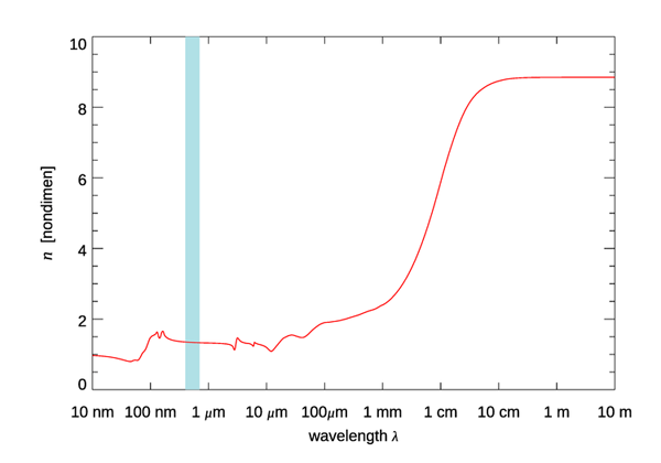
Pay attention to the frequency dependence when comparing and values. If you look up the values of and for water in a freshman physics text, it will probably show the values as (e.g., Halliday and Resnick (1988), page 867) and (ibid. page 627). Figure 1 shows the index of refraction of pure water as a function of wavelength. At the long wavelength/low frequency end of the spectrum, corresponding to , which is the value for room temperature water. (The value of is temperature dependent and at low frequencies decreases from about 88 at 0 C to about 56 at 100 C.) At visible wavelengths, is around 1.77 and is around 1.33, consistent with . There are small temperature, salinity, and pressure effects on at the visible wavelengths of interest here; see the Water page for formulas and tables.
Scattering Models
As stated above, elastic scattering occurs when light travels from a region with one index of refraction into a region with a different index of refraction. In this sense, all scattering is the same. However, there are many ways in which the index of refraction can change, which leads to many ways to model the resulting scattering. You will sometimes see terms like “surface scattering” or “volume scattering.” Surface scattering refers to scattering caused by a change in index of refraction at the boundary between two media, such as at the air-water interface. Volume scattering refers to scattering caused by a change in index of refraction within a medium, such as a water body. Volume scattering can be caused by the presence of discrete particles embedded in the medium, by thermal fluctuations in density, or by turbulent mixing of fluids with different physical properties. Those classifications can be useful, but they also can be misleading because they make it seem like there are many unrelated types of scattering, when in reality the terms just describe different ways to change the index of refraction.
Reflection and Refraction: Snell’s Law
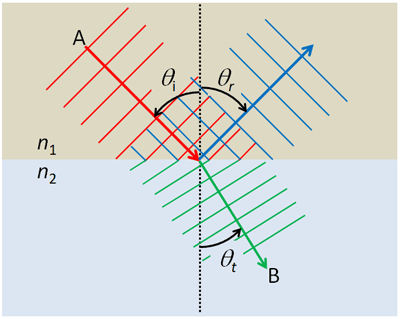
The easiest scattering to model is reflection and refraction at a dielectric interface, such as a level air-water surface. At the level of freshman physics, this is usually explained in terms of a plane wave incident onto a boundary between two dielectrics with indices of refraction and as illustrated in Fig. 2. The red lines in the figure represent lines of constant wave phase, and the red arrow shows the direction of light propagation. The light in medium 1 propagates at a speed of , where is the speed of light in a vacuum; in medium 2 the propagation speed is . If , the wave slows down as the incident wave front enters medium 2. This causes the wave front to change direction as it enters medium 2, as shown by the green lines and arrow. The frequency of the wave remains unchanged as the wave passes from medium 1 to 2. Therefore, the wavelength in medium 2 must be less than the wavelength in medium 1: .
The relationship between the indices of refraction and the angles of incidence, , and refraction or transmission, , was empirically discovered by the Persian Abu Ibn Sahl who reported his discovery in a book On Burning Mirrors and Lenses published in Bagdhad in 984. Ibn Sahl even used his discovery to design the shapes of lenses that would focus parallel light rays without abberation. The same result was rediscovered in 1621 by Willebrord Snel van Royen (note the spelling of his name), who published in Latin under the name Snellius. After Latin was replaced first by German and then English as the common language of western science, Snellius became Snell. Unfortunately, Ibn Sahl’s book was unknown in the west until its rediscovery in the 1930s, so the law became known as Snell’s law, although the Ibn Sahl-Snel law would be a more appropriate name. Regardless of what it is called, the relation between the angles of incidence and transmission is given by
| (1) |
The surface also reflects some of the incident light back into medium 1, as shown by the blue lines and arrow in Fig. 2. For reflection,
| (2) |
which is known as the law of reflection.
Snell’s law can be derived from fundamental physics at various levels of understanding. One derivation follows from Fermat’s Principle of Least Time, which says that light traveling from point A to point B will follow the path that takes the least time. Applied to the geometry of Fig.2, this gives the ray path that obey’s Snell’s law. (To be honest, Fermat cooked up his principle as a way to explain Snell’s law, but the principle turns out to have greater applicability.)
Snell’s law can be rigorously derived from Maxwell’s equations by solving the equations for a plane wave incident onto a dielectric interface. This problem is formulated in terms of the electric fields of the incident, reflected, and transmitted plane waves, and full account is made of the state of polarization of the plane waves. That is a nasty bit of physics and mathematics (e.g., Griffiths (1981) Section 8.2.5 or Feynman et al. (1964) Chapter 33). However, the effort required to solve Maxwell’s equations pays off well because the solution gives not just Snell’s law, which gives only the directions of light propagation, but also Fresnel’s Equations, which give the magnitudes of the reflected and transmitted fields (i.e., of the irradiances) accounting for the state of polarization of the incident light. This solution also shows that the incident, reflected, and transmitted rays must lie in the same plane. The three results of (1) Snell’s law, (2) the law of reflection, and (3) the coplanar geometry of the rays are the essence of geometric or ray-tracing optics.
The index of refraction is a bulk material property that parameterizes the accumulated effects of how light interacts with the individual atoms that make up the material. For the most fundamental understanding, Feynman (1985) outlines how Snell’s law arises from the properties of individual photons and atoms interacting via the laws of Quantum Electrodynamics (see The Nature of Light).
Fortunately, for oceanographic purposes, we can just accept Eqs. (1) and (2) and Fresnel’s equations and carry on with their applications such as predicting the reflectance and transmittance of wind-blown sea surfaces, as described beginning at The Level Surface.
Scattering by Homogeneous Spheres: Mie Theory
Another way to change the index of refraction is to imbed a particle of some index of refraction within a medium with a different index of refraction. If the imbedded particle is a homogeneous sphere (of any radius), the solution of Maxwell’s Equations for a plane wave incident onto the sphere is called Mie Theory. The problem is formulated as follows.
- We have given a single, homogeneous sphere of radius , whose material is a dielectric with a complex index of refraction . Here is the real index of refraction, and is the complex index of refraction. The complex index is related to the absorption coefficient of the sphere material by , where is the wavelength in vacuo corresponding to the frequency of an electromagnetic wave.
- The sphere is imbedded in a non-absorbing, homogeneous, infinite medium whose real index of refraction is .
- A plane electromagnetic wave of frequency is incident onto the sphere. The wavelength on the incident light in the medium is thus , which corresponds to a wavelength in vacuo of .
- We wish to find the electric field within the sphere and throughout the surrounding medium. That is, we wish to determine how the incident light is absorbed and scattered by the sphere, including the angular distribution of the scattered light and its state of polarization.
The solution of this geometrically simple problem is exceptionally difficult. Indeed, this is one of the classic problems of applied mathematics, and its solution was attempted (and partially achieved in various forms) by many of the most illustrious figures of nineteenth-century physics. For historical reasons, Mie (1908) usually gets credit for the complete solution of the problem, and his solution of Maxwell’s equations is commonly called Mie Theory. Mie’s paper is 69 pages of dense equations, and I doubt that more than a handful of people have actually read the entire paper, although it has been cited in thousands of papers. Bohren and Huffman (1983) say (on page 93) that someone who works through the details of Mie’s solution will have “acquired virtue through suffering.” The details of Mie’s solution are given in the texts by van de Hulst (1957) and by Bohren and Huffman (1983). An overview of Mie theory is given on the Level 2 page Mie Theory Overview, and example output from Mie calculations is given on the Mie Theory Examples page.
Mie Theory is exact and valid for all sizes of spheres, indices of refraction, and wavelengths. Unfortunately, the solution is in the form of infinite series of complicated mathematical functions. The terms in these series depend on a size parameter ,
| (3) |
and on the complex refractive index of the sphere relative to that of the surrounding medium,
| (4) |
The size parameter is a measure of the sphere’s size relative to the wavelength of the incident light in the surrounding medium. This parameter shows why oceanographers tend to use wavelength rather than frequency as the measure of light’s oscillations: it is particle size relative to wavelength that is important for scattering (whether or not the particle is spherical). Note that the real paft of the relative refractive index can be less than 1, for example if the spherical particle is an air bubble () in water ().
Because of its computational complexity, Mie’s solution was of little use until computers became readily available in the 1960s. However, once it became possible to compute the sums of the infinite series with good accuracy, Mie theory found applications in all fields where scattering by particles is important. One of the first of computer codes, and still perhaps the most widely used, is the BHMIE code given in Appendix A of Bohren and Huffman (1983). There are now programs available in all commonly used scientific computer languages (Fortran, C, MATLAB, IDL, and Python). See, for example, the websites at SCATTERLIB and Codes for Electromagnetic Scattering by Spheres. There are also online Mie calculators that are useful if you only want to obtain a few solutions for small size parameters. See for example Scott Prahl’s Mie Scattering Calculator, which is an excellent place to explore Mie Theory. If you need to get serious about doing lots of Mie calculations, download one of the Fortran codes. As Prahl notes on his website, “Let me state that the best Mie codes are in Fortran. Period.”
The output of Mie codes is usually given as various absorption and scattering efficiencies. The absorption efficiency , for example, gives the fraction of radiant energy incident on the sphere that is absorbed by the sphere. The term “energy incident on the sphere,” means the energy of the incident plane wave passing through an area equal to the cross-sectional (projected, or “shadow”) area of the sphere, . Likewise, the total scattering efficiency gives the fraction of incident energy that is scattered into all directions. Other efficiencies can be defined: for total attenuation, for backscattering, and so on.
Mie solutions also can be presented in terms of absorption and scattering cross sections. The physical interpretation of these cross sections is simple. The absorption cross section , for example, is the cross sectional area of the incident plane wave that has energy equal to the energy absorbed by the sphere. The absorption and scattering cross sections are therefore related to the corresponding efficiencies by the geometrical cross section of the sphere. Thus
Likewise, , and so on for , etc.
Mie codes also output the scattering phase function . However, Mie codes usually output unnormalized phase functions, so you must always integrate a phase function to verify its normalization. Keep in mind that a phase function must satisfy the normalization before it can be used in HydroLight. This is discussed in more detail on the Mie Theory Examples page.
Understanding the Mie output sometimes involves the nondimensional phase-shift parameter
and the nondimensional absorption thickness
It is important to note, when computing the absorption thickness , that is the absorption coefficient of the sphere material, not the bulk absorption coefficient of the medium (e.g., of seawater plus phytoplankton). Phytoplankton cells typically have values of - at visible wavelengths. (Think of the highly absorbing chlorophyll in a phytoplankton cell as the chlorophyll in a can of chopped spinach; you do not see very far through solid spinach.) As an example of the Mie parameter values, consider a phytoplankton cell with , , and . If the cell is floating in water with , and if the incident light has in vacuo, then , and .
Scattering by Irregular Particles
Strictly speaking, Mie theory is applicable only to homogeneous spherical particles. That of course does not keep it from being misapplied to non-spherical and/or non-homogeneous particles. Such particles are common in nature: chain-forming or non-spherical diatoms, ice crystals in cirrus clouds, atmospheric dust, and resuspended sediments in water. Fortunately, Mie theory often gives a useful approximate solutions to scattering by irregular particles so long as the particles are close to spherical, such as prolate or oblate spheroids. There are many applications where people use Mie theory with an “equivalent” spherical particle, where the equivalent particle is given the same volume (or cross sectional area) as the irregular particle of interest. For equivalent-volume, roughly spherical particles, Mie may work well. However, for very irregular particles, Mie predictions may disagree greatly with measurements made on such particles. The differences in phase functions between spherical and non-spherical particles are often greatest at backscattering directions, which are of great interest for remote sensing.
In one sense, every spherical particle is geometrically the same; the spheres differ only in size and index of refraction. Thus Mie theory requires only the size parameter and the relative index of refraction as inputs. However, irregular particles can have any imaginable shape and composition. This makes it impossible to have a solution technique for Maxwell’s equations that requires only simple inputs.
Many numerical techniques have been developed to compute scattering by irregular particles, all of which are exceedingly mathematical; see Computational Electromagnetics for an introduction. The two most widely used techniques are probabtly the T-matrix Method (e.g., Mishchenko et al. (2002), Chapter 5) and the Discrete Dipole Approximation. Although computer codes are available to perform the calculations (SCATTERLIB), they are not trivial to use. In particular, you must first build in the geometry of the particle shape of interest, which in itself can be a major undertaking. For a collection of randomly oriented particles, scattering must first be computed for each possible particle orientation, and then the results must be averaged over all possible particle orientations.
If the irregular particle is much larger than the wavelength of light (e.g., an ice crystal in a cirrus cloud or a large sand grain in the ocean), then geometric optics and ray tracing can be used as the core of Monte Carlo simulations of many rays incident onto randomly oriented particles. As always, you must first program the logic defining the particle shape and how to determine when a ray intersects the surface of the particle (this is non-trivial even for simple particle shapes like cubes). But after that is done, it is just a matter of computer time until enough rays have been traced to give good statistical results.
Enough has now been said about scattering by particles for this overview page. The point to be remembered is that a particle is just a discontinuity in a medium’s index of refraction. If you insert a relative index of refract of into Mie or T-matrix theory, you get no scattering because the particle’s properties then match those of the surrounding medium. In essence, a non-absorbing particle becomes invisible.
Scattering by Pure Water: Einstein-Smoluchowski Theory
When computing scattering by particles, the surrounding medium is viewed as a continuous, homogeneous medium that itself does not scatter. However, even the purest of water has some scattering. This is because, at the atomic level, pure water is composed of particles, namely water molecules. In water at room temperature, the water molecules are moving on average at about and are continually bumping into each other and flying apart in random directions. These molecular motions are continually creating small volumes of water that for a very short time have more or fewer molecules per cubic meter than on average. These fluctuations in the number density of water molecules create small-scale fluctuations in the index of refraction.
The phenomenon of critical opalescence refers to a transparent gas or liquid becoming foggy and opaque near a continuous (second-order) phase transition (such when a gas and liquid can coexist at sufficiently high temperature and pressure). An explanation of this phenomenon was lacking until the papers of Smoluchowski (1908) and Einstein (1910). They showed that large thermodynamic fluctuations in the material’s density, hence in the index of refraction, are responsible for the optical scattering that makes the substance become cloudy. Their explanation required a sophisticated combination of thermodynamics, statistical mechanics, and electromagnetic theory (Maxwell’s equations). [Or so I’m told. Wyley, which now owns the journal Annalen der Physik where the papers were published, wants $49 each to download pdfs of these classic papers. I find that unconscionable for papers over a century old, so I haven’t actually read these papers.]
The same process applies to ordinary scattering by water molecules, for which the density fluctuations are much smaller but still non-zero. In this case, the Einstein and Smoluchowski formula for the volume scattering function, with later modifications to account for polarization effects, is
| (5) |
The terms in this equation are as follows, with values shown for a temperature of 20 C, pressure of one atmosphere, and wavelength of 546 nm, as obtained from the formulas of Buiteveld et al. (1994):
- Boltzman’s constant;
- Temperature;
- Index of refraction;
- Isothermal compressibility of water:
- Isothermal pressure derivative of the index of refraction;
- depolarization ratio; 0.031 (from Zhang et al. (2019))
- wavelength;
- pressure;
- polar scattering angle
The temperature-dependent fluctuations in the index of refraction appear in Eq. (5) via the various thermodynamic quantities. The equation shows that scattering will be stronger for a higher temperature; this is because the random molecular motions are then greater, and consequently the density fluctuations are larger. The more compressible a fluid is, the greater the density fluctuations, and the greater the scattering. In particular, if the index of refraction did not depend on the pressure, would be zero and there would be no scattering. The scattering is strongly dependent on wavelength, with shorter wavelengths scattering much more strongly than long wavelengths. The wavelength dependence seen in (5) is the same as for Rayleigh scattering, which describes scattering by spheres that are much smaller than the wavelength of light (and which can be obtained from Mie theory when the particle size is much less than the wavelength of the light). The same wavelength dependence occurs here because in ordinary water the spatial size of the density fluctuations is much less than the wavelength of visible light.
Inserting the values just listed into Eq. (5) gives, for a scattering angle of ,
This is within a few percent of the value of the often-cited value of 0.83 measured by Morel (1974). Further discussion of the best values for the various inputs to Eq.(5) is given in Zhang and Hu (2009) and Zhang et al. (2019).
Finally, it must be pointed out that scattering by pure water (or pure sea water if salinity effects are included in the index of refraction) is one of the few IOPs that can be computed from fundamental physics. (Another such IOP is scattering by a homogeneous sphere, computed using Mie theory.) Other IOPs, absorption coefficients in particular, are obtained from measurements and not from fundamental physics.
Scattering by Turbulence
Yet another way to change the index of refraction is via turbulence-induced fluctuations in temperature and salinity, with the water being viewed as a continuous but slightly inhomogeneous medium. The temperature and salinity fluctuations generate small-scale but spatially continuous changes in the index of refraction, which in turn cause small-angle deviations in the direction of light propagation. Such deviations cause “beam wander” in laser beams and can degrade visibility, which is affected by small-angle scattering. Such effects are often called “optical turbulence.” In the atmosphere, optical turbulence is responsible for the twinking of stars or the shimmering image of a distant object viewed on a hot day.
We can get an order-of-magnitude estimate of the size of the turbulence-induced fluctuations in the real index of refraction as follows. Hold the wavelength and pressure constant, so that is a function only of the temperature and salinity . (Water is almost incompressible, which makes the pressure dependence of much less than that of temperature and salinity.) Then taking differentials of gives
where and are small fluctuations in and , and is the corresponding change in . If we square this equation, average it over many turbulent fluctuations, and assume that the fluctuations in temperature and salinity are uncorrelated, we obtain
| (6) |
Here represents the average of the enclosed quantity. The root-mean-square (rms) value of the index-of-refraction fluctuations is then . The derivatives and must be evaluated at particular values of and . We can estimate typical values from from the tabulated data in Austin and Halikas (1976). (Some of their data are shown in Table 2 of the Water page, and in Figure 3.5 of Light and Water (1994) Figure 3.5.) Let us take , and . Then from the tabulated data of Austin and Halikas (their page A-6)
Now let us suppose that the temperature and salinity fluctuations are of magnitude and . Then Eq. (6) gives
The turbulence-induced fluctuations in the index of refraction are therefore on the order of parts per million.
Such small changes in are negligible compared to the 3% “fluctuation” in when light encounters a plankton cell with (relative to the water). However, in the case of particle scattering, we envision the light traveling in straight lines between the occasional encounter with a particle, at which time there may be a large change in direction. In the case of turbulence, we envision many turbulent blobs of water, of many sizes, with the light slightly but continuously changing direction as it passes through water with a continuously varying index of refraction. It is then possible for the cumulative effect of the turbulent fluctuations to change a light’s direction by a fraction of a degree. These turbulence-induced deviations manifest themselves in time-averaged scattering measurements as large values of the VSF at very small scattering angles.
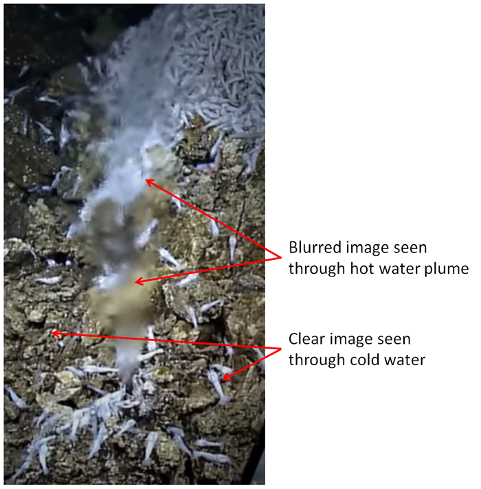
Turbulence-induced scatter can significantly degrade the quality of underwater images. The effects of turbulence are especially noticeable in video photography, since the time dependence of the random fluctuations is then apparent, just as it is with the twinkling of stars caused by atmospheric turbulence. Near the boundary between distinctly different water masses, the fluctuations in and can be much larger than those assumed above, and even still images can be badly degraded. Fluctuations in and can be very large— of many degrees and of many PSU—when cold and/or fresh water mixes with warm and/or salty water. This can occur when rain falls on the sea surface, where rivers enter the ocean, and near hydrothermal vents at the sea floor. In these extreme cases, optical turbulence near the boundary of the two mixing water masses can cause striking visual effects such as shimmering of objects see through the water mass boundary. Figure 3 shows and example of this. The fluid being expelled by a hydrothermal vent can be as hot as 350 C, in which case the turbulence-induced fluctuation in is comparable to the change in caused by a phytoplankton.
Turbulence effects on optics have been intensively studied by the atmospheric optics community, but less studied by the hydrologic optics community. This is often justified because the turbulence-induced changes in within water bodies usually are very small and do not significantly effect the distribution of radiant energy within the water. The exception is found in the community of researchers interested in high-resolution underwater visibility and imaging, and in the behavior of coherent light beams. Because the time-averaged effects of turbulence are included in measured volume scattering functions, we can assume that those effects are accounted for in the highly peaked VSFs used for oceanic radiative transfer modeling.
 See comments posted for this page and leave your own.