Page updated:
February 3, 2021
Author: Curtis Mobley
View PDF
HydroLight
Full disclosure: HydroLight was developed by web book author Curtis Mobley and is a commercial software product of Numerical Optics, Ltd.
HydroLight is a radiative transfer numerical model that computes radiance distributions and derived quantities (irradiances, reflectances, K functions, etc.) for natural water bodies. It is designed to solve a wide range of problems in optical oceanography and ocean color remote sensing. Many of the pages of this web book show HydroLight-computed results.
In brief, HydroLight solves the time-independent, depth-dependent, scalar radiative transfer equation (Eq. 3 of the SRTE page) to compute the radiance distribution within and leaving any plane-parallel water body. The spectral radiance distribution is computed as a function of depth, direction, and wavelength within the water. The upwelling radiance just above the sea surface includes both the water-leaving radiance and that part of the incident direct and diffuse sky radiance that is reflected upward by the wind-blown sea surface. The water-leaving and reflected-sky radiances are computed separately in order to isolate the water-leaving radiance, which is the quantity of interest in most remote sensing applications. Input to the model consists of the absorbing and scattering properties of the water body, the nature of the wind-blown sea surface and of the bottom of the water column, and the sun and sky radiance incident on the sea surface. Output consists both of archival printout and of files of digital data from which graphical, spreadsheet, or other analyses can be performed.
The input absorbing and scattering properties of the water body can vary arbitrarily with depth and wavelength. These IOPs can be obtained from actual measurements or from analytical models, which can build up the IOPs from contributions by any number of components. The software comes with various bio-optical models for Case 1 and 2 waters, which are based on historical and recent publications on absorption and scattering by various water constituents. The most general case 2 IOP model can have any number of components (such as different phytoplankton functional groups, different types of mineral particles, dissolved substances, bubbles, etc.). The user can also write subroutines to define the IOPs in any chosen way.
The input sky radiance distribution can be completely arbitrary in the directional and wavelength distribution of the solar and diffuse sky light. HydroLight does not solve the RTE for the atmosphere to obtain the radiance incident onto the sea surface. However, it does include default sky radiance and irradiance models based on published atmospheric radiative transfer models.
In its most general solution mode, HydroLight includes the effects of inelastic scatter by chlorophyll fluorescence, by colored dissolved organic matter (CDOM) fluorescence, and by Raman scattering by the water itself. The model also can simulate internal layers of bioluminescing microorganisms.
HydroLight employs mathematically sophisticated invariant imbedding techniques to solve the radiative transfer equation. Details of this solution method are given in Light and Water (1994). When computing the full radiance distribution, invariant imbedding is computationally extremely fast compared to other solution methods such as discrete ordinates and Monte Carlo simulation. Computation time is almost independent of the depth variability of the inherent optical properties (whereas a discrete ordinates model, which resolves the depth structure as N homogeneous layers, takes N times as long to run for stratified water as for homogeneous water). Computation time depends linearly on the depth to which the radiance is desired (whereas Monte Carlo computation times increase exponentially with depth). All radiance directions are computed with equal accuracy. There is no statistical noise caused by the invariant imbedding in-water RTE solution (although there can be a small amount of statistical noise resulting from HydroLight’s Monte Carlo treatment of wind-blown water surfaces). Monte Carlo models suffer from statistical noise, and quantities such as radiance contain more statistical noise than quantities such as irradiance, because the simulated photons must be partitioned into smaller directional bins when computing radiances. The water-leaving radiance—the fundamental quantity in remote sensing studies—is very time consuming to compute with Monte Carlo simulations because so few incident photons are backscattered into upward directions.
HydroLight has been under development for over 30 years, with its first published description in Mobley (1989). It has been extensively compared with independent numerical models, e.g., in Mobley et al. (1993, wherein HydroLight version 3.0 is referred to as “Invariant Imbedding”). The literature contains many comparisons between HydroLight predictions and measurements in hundreds of publications than have used HydroLight in one way or another. Representative examples are seen in Mobley et al. (2002), Chang et al. (2003), and Tzortziou et al. (2006). Although several researchers have developed excellent numerical codes for solving the RTE in the oceanographic setting, their codes are not readily available. HydroLight is commercially available and therefore is widely used.
The HydroLight Physical Model
The version of the RTE solved by HydroLight is describes the following physical conditions:
- time-independent
- horizontally homogeneous IOPs and boundary conditions
- arbitrary depth dependence of IOPs
- wavelengths between 300 and 1000 nm (for the default underlying databases)
- sea surfaces are modelled either by wave variance spectra or by Cox-Munk capillary-gravity wave sea-surface slope statistics
- finite or infinitely deep (non-Lambertian) water-column bottom
- can optionally include Raman scatter by water
- can optionally include fluorescence by chlorophyll and CDOM
- can optionally include horizontally homogeneous internal sources such as bioluminescing layers
- includes all orders of multiple scattering
- does not include polarization
- does not include whitecaps
These conditions are appropriate for many (but not all) oceanographic simulations. HydroLight cannot, for example, simulate time-dependent wave focusing by surface waves because its sea surface treatment describes the spatially or temporally averaged effects of surface waves. It cannot be user for pulsed Lidar bathymetry simulation, which is an inherently time-dependent problem. It cannot simulate sloping bottoms or the radiance reflected by an object in the water, which are inherently 3D problems. Probably the most limiting simplification of the physics of HydroLight is that it solves the scalar, or unpolarized, RTE. It thus cannot be used for studies where the state of polarization is of interest.
The HydroLight Computational Model
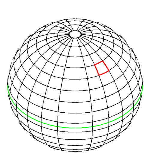
Any radiance sensor actually measures an average of taken over some finite solid angle , which is determined by the field of view of the instrument, and over some finite bandwidth , which is determined by the wavelength response of the instrument. Likewise, in order to solve the RTE numerically, it must be discretized (or otherwise simplified) by averaging over direction and wavelength to obtain a finite number of values that must be computed. In HydroLight, this directional averaging is performed by first partitioning the set of all directions , into regions bounded by lines of constant (like lines of constant latitude) and constant (constant longitude), plus two polar caps. These quadrilateral regions and polar caps are collectively called “quads.” The individual quads are labeled by discrete indices and to show their and positions, respectively. The standard (default) quad layout is shown in Figure 1. In this layout, which has and , the polar caps have a 5 deg half angle and the boundaries lie at 5, 15, 25, ...,75, 85, 90, 95, 105, ..., 175 deg. For mathematical reasons there is no quad centered on the “equator” at . However, the radiances computed for the 85-90 and 90-95 deg quads can be averaged to get the “horizontal” radiance at a nominal angle of . Thus the HydroLight standard quad layout essentially gives 10 deg resolution in and 15 deg in . This is adequate for most oceanographic simulations.
Similarly, the wavelength region of interest is partitioned into a number of contiguous wavelength bands of width . The need not be the same size for different j values.
The fundamental quantities computed by HydroLight are then the quad- and band-averaged radiances at any selected set of depths :
The quads “homogenize” or average the radiance within each quad, just like a diffuser does in an instrument. Thus, in the quad layout of Fig. 1, it is not possible to resolve the difference in the radiance for polar angles and , because they both lie in the same quad extending from and . However, there is a difference in and , because those angles lie in different quads and thus are represented by (probably) different quad-averaged radiances. This same sort of directional averaging of radiances occurs in Monte Carlo models, which collect rays in directional “bins.” If it is necessary to have greater angular resolution in the radiance distribution, a different quad layout can be created. However, the computer storage and run time are proportional to the square of the number of quads, so increasing the angular resolution comes with increased computational cost, just as for other solution techniques.
Ways in Which HydroLight Can Be Used
HydroLight has been used in numerous published studies on topics as diverse as biological primary production, ecosystem modeling, remote sensing, underwater visibility, mixed-layer thermodynamics, and the generation of large synthetic data sets needed for neural network training, spectrum-matching libraries, and design of ocean color satellite sensors and retrieval algorithms. These studies have used HydroLight in various ways:
- HydroLight can be run with modeled input values to generate in-water scalar irradiances, which in turn become the input to models of primary productivity or mixed-layer thermodynamics. Accurate light calculations are fundamental to the coupling of physical, biological, and optical ecosystem models.
- HydroLight can be run with the IOP’s of different water types to simulate in-water light fields for the purpose of selecting or designing instruments for use in various water types. Such information aids in the planning of field experiments.
- HydroLight can be run with assumed water inherent optical properties as input, in order to obtain estimates of the signals that would be received by various types or configurations of remote sensors, when flown over different water bodies and under different environmental conditions. Such information can guide the planning of specific operations.
- HydroLight can be used to isolate and remove unwanted contributions to remotely sensed signatures. Consider the common remote-sensing problem of extracting information about a water body from a downward-looking imaging spectrometer. The detected radiance contains both the water-leaving radiance (the signal, which contains information about the water body itself) and sky radiance reflected upward by the sea surface (the noise). HydroLight separately computes each of these contributions to the radiance heading upward from the sea surface and thus provides the information necessary to correct the detected signature for surface-reflection effects.
- When analyzing experimental data, HydroLight can be run repeatedly with different water optical properties and boundary conditions, to see how particular features of the data are related to various physical processes or features in the water body, to substance concentrations, or to boundary or other external environmental effects. Such simulations can be valuable in formulating hypotheses about the causes of various features in the data.
- HydroLight can be used to simulate optical signatures for the purpose of evaluating proposed remote-sensing algorithms for their applicability to different environments or for examining the sensitivity of algorithms to simulated noise in the signature.
- HydroLight can be used to characterize the background environment in an image. When attempting to extract information about an object in the scene, all of the radiance from the natural environment may be considered noise, with the radiance from the object being the signal. HydroLight can be used to compute and remove the environmental contribution to the image.
- HydroLight can be run with historical (climatological) or modeled input data to provide estimates about the marine optical environment during times when remotely or in-situ sensed data are not available.
Inputs to HydroLight
In order to run HydroLight to predict the spectral radiance distribution within and leaving a particular body of water, during particular environmental (sky and surface wave) conditions, the user supplies the core model with the following information (via built-in submodels, or user-supplied subroutines or data files):
- The inherent optical properties of the water body. These optical properties are the absorption and scattering coefficients and the scattering phase function. These properties must be specified as functions of depth and wavelength.
- The state of the wind-blown sea surface. HydroLight models the sea surface using the Cox-Munk capillary-gravity wave slope statistics, which adequately describe the optical reflection and transmission properties of the sea surface for moderate wind speeds and solar angles away from the horizon. In this case, only the wind speed needs to be specified.
- The sky spectral radiance distribution. This radiance distribution (including background sky, clouds, and the sun) can be obtained from semi-empirical models that are built into HydroLight, from observation, or from a separate user-supplied atmospheric radiative transfer model (such as MODTRAN).
- The nature of the bottom boundary. The bottom boundary is specified via its bidirectional reflectance distribution function (BRDF). If the bottom is a Lambertian reflecting surface at a finite depth, the BRDF is defined in terms of the irradiance reflectance of the bottom. For infinitely deep water, the inherent optical properties of the water body below the region of interest are given, from which HydroLight computes the needed (non-Lambertian) BRDF describing the infinitely deep layer of water below the greatest depth of interest.
The absorption and scattering properties of the water body can be provided to HydroLight in various ways. For example, if actual measurements of the total absorption and scattering are available at selected depths and wavelengths, then these values can be read from files provided at run time. Interpolation is used to define values for those depths and wavelengths not contained in the data set. In the absence of actual measurements, the IOPs of the water body can be modeled in terms of contributions by any number of components. Thus the total absorption can be built up as the absorption by water itself, plus the absorption by chlorophyll-bearing microbial particles, plus that by CDOM, by detritus, by mineral particles, and so on. In order to specify the absorption by chlorophyll-bearing particles, for example, the user can specify the chlorophyll profile of the water column and then use a bio-optical model to convert the chlorophyll concentration to the needed absorption coefficient. The chlorophyll profile also provides information needed for the computation of chlorophyll fluorescence effects. Each such absorption component has its own depth and wavelength dependence. Similar modeling can be used for scattering.
Phase function information can be provided by selecting (from a built-in library) a phase function for each IOP component, e.g., using a Rayleigh-like phase function for scattering by the water itself, by using a Petzold type phase function for scattering by particles, and by assuming that dissolved substances like CDOM do not scatter. HydroLight can also generate phase functions that have a specified backscatter fraction. For example, if the user has both measured scattering coefficients (e.g., from a WETLabs ac-s instrument) and measured backscatter coefficients (e.g., from a WETLabs bb-9 or HOBILabs HydroScat-6 instrument), then HydroLight can use the ratio to generate a Fournier-Forand phase function that has the same backscatter fraction at each depth and wavelength. The individual-component phase functions are weighted by the respective scattering coefficients and summed in order to obtain the total phase function.
HydroLight does not carry out radiative transfer calculations for the atmosphere per se. The sky radiance for either cloud-free or overcast skies can be obtained from simple analytical models or from a combination of semi-empirical models. Such models are included in the HydroLight code. Alternatively, if the sky radiance is measured, that data can be used as input to HydroLight via a user-written subroutine. It is also possible to run an independent atmospheric radiative transfer model (such as MODTRAN) in order to generate the sky radiance coming from each part of the sky hemisphere, and then give the model-generated values to HydroLight as input.
The bottom boundary condition is applied at the deepest depth of interest in the simulation at hand. For a remote sensing simulation concerned only with the water-leaving radiance, it is usually sufficient to solve the radiative transfer equation only for the upper two optical depths, because almost all light leaving the water surface comes from this near-surface region. In this case, the bottom boundary condition can be taken to describe an optically infinitely deep layer of water below two optical depths. In a biological study of primary productivity, it might be necessary to solve for the radiance down to five (or more) optical depths to reach the bottom of the euphotic zone, in which case the bottom boundary condition would be applied at that depth. In such cases, HydroLight computes the needed bottom boundary BRDF from the inherent optical properties at the deepest depth of interest. The bottom boundary condition also can describe a physical bottom at a given geometric depth. In that case, irradiance reflectance of the bottom must be specified (for a Lambertian bottom). In general, this reflectance is a function of wavelength and depends on the type of bottom—mud, sand, sea grass, etc. The user can also supply a subroutine to define a non-Lambertian bottom BRDF.
Output from HydroLight
HydroLight generates files of archival “printout,” which are convenient for a quick examination of the results, and larger files of digital data. The digital files include Excel spreadsheets and files of data (including the full radiance distribution) formatted for input into graphics packages such as IDL. (The software package contains example routines that use IDL to read and plot HydroLight output. Those routines created many of the HydroLight-computed figures in the web book pages.). The default printout gives a moderate amount of information to document the input to the run and to show selected results of interest to most oceanographers (such as various irradiances, reflectances, mean cosines, K-functions, and radiances in selected directions). This output is easily tailored to the user’s requirements. A file of digital data contains the complete input and output for the run, including the full radiance distribution. This file is generally used as input to plotting routines that give graphical output of various quantities as functions of depth, direction, or wavelength. All input and output files are in ASCII (text file) format to enable easy transfer between different computer systems.
Documentation
The invariant imbedding algorithms used within HydroLight are described in detail in Light and Water (1994), in particular Chapters 4 and 8. The source code is extensively documented with comments referencing equations in Light and Water and other publications. There is a Users’ Guide that describes how to run the code, and Technical Documentation that gives information about the included models for IOPs, bottom reflectances, sky radiances, and such. The latest versions of these documents can be downloaded from the references page.
The software itself comes in native versions for the Microsoft Windows, Apple OSX, and Linux operating systems. The mathematical source code is written in Fortran 95. The user interface is written in C++ and uses the Qt library for graphical elements. There are related specialized versions of HydroLight called EcoLight and EcoLight-S(ubroutine). For further details, see Numerical Optics, Ltd..
Caveat Emptor: There are many “HydroLight” products on the market, including hydrogen powered lighting systems, hydroelectric power systems, underwater dive lights, lighting for irrigation systems, lighting for growing recreational plants in your basement hydroponics tank, and even skin care lotions, bicycles, sports drinks, and a toothbrush. However, none of those other HydroLights can solve the radiative transfer equation.
 See comments posted for this page and leave your own.