Page updated:
March 22, 2021
Author: Curtis Mobley
View PDF
Numerical Resolution
The question naturally arises: “How large a region and how many points must be used in generating sea surface realizations?” Not surprisingly, the general answer is, “It depends on your application.” It is computationally possible to create 2-D surfaces with sufficiently large values in the and directions, but run times are prohibitive. Kay et al. (2011) created 2-D surfaces with = points in each dimension, which sampled the variance spectrum for wavelengths from 200 m gravity waves to 3 mm capillary waves. However, it took 6 hours to create just one surface on a 3 GHz computer. Note also that the storage of this surface requires numbers. Many ray tracing applications need to use tens of thousands of surface realizations to get good statistical averages. Thus, the specific answer for brute-force scientific calculations is usually, “A bigger than you can run on your computer.” This page shows one way to finesse certain calculations so that large- calculations can be avoided.
For creating visually appealing sea surfaces for rendering into a movie scene, or perhaps at most is usually adequate. This is because the visual impression of a sea surface is, to first order, determined by the height of the waves, which in turn is governed by the largest gravity waves for the given wind speed. If you are rendering an image, you don’t need to have a finer resolution for the sea surface than maps to an image pixel. For example, if you are going to simulate what a CCD with pixels would record, and you are looking down onto the sea surface from above at an elevation where one CCD pixel sees a patch of the sea surface, then you need to resolve the sea surface with a grid spacing of at most 0.1 m. Modeling a patch of sea surface with a spatial resolution of gives a grid spacing of 0.1 m, which would be adequate for the CCD image simulation.
Unfortunately, for accurate scientific calculations of sea surface reflectance, may have to be much larger. This is because the surface reflectance depends to first order on the surface wave slope, and the slope is strongly affected by the smallest waves with spatial scales down to capillary size of a few millimeters.
The value of the peak of the Pierson-Moskowitz spectrum
| (1) |
is easily obtained from setting and solving for the value of . This gives
which corresponds to a wavelength of . Table shows the values of and for a few wind speeds.
| ] | ||
| 5 | 0.276 | 23 |
| 10 | 0.069 | 91 |
| 15 | 0.031 | 205 |
| 20 | 0.017 | 364 |
If we use for the size of the spatial domain, we will resolve the large gravity waves, which contain most of the wave variance. (Keep in mind that density functions do not have a unique maximum: the location of the maximum of a density function depends on which frequency variable is chosen. See the discussion of this on the page A Common Misconception. Differentiating the Pierson-Moskowitz spectrum
| (2) |
and using the dispersion relation leads to , which gives 73 m at . However, either version of gives adequate guidance for our present purpose.)
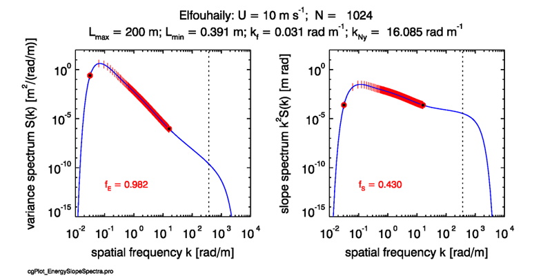
Now consider how many points it takes to almost fully resolve, or account for, the variances of elevation and slope spectra when they are sampled for a DFT. For a specific example, take and and use the omnidirectional, or 1-D, part of the Elfouhaily et al. spectrum presented on page Wave Variance Spectra: Examples. This is given by Eq. (5) and the associated equations on that page. This variance spectrum and the corresponding slope spectrum are plotted as the blue curves in the next 3 figures.
As we have learned on page Wave Variance Spectra: Theory, the expected variance of the sea surface is given by
| (3) |
and the mean-square slope is given by
| (4) |
Such integrals usually must be numerically evaluated with the limits of and being replaced by some small value and some large but finite value . The present example uses and , with evaluation points in between these limits. That gives an accurate evaluation of Eqs. (3) and (4) for the spectra. The results are and .
Now suppose we sample the spectrum using points, which leads eventually to a sea surface realization with 1024 points. For the fundamental frequency is . This point is shown by the left-most red dot with the black center in Fig. 1. For this and , the Nyquist frequency is , which is shows by the right-most black and red dot. These two end points and the red vertical lines in between show the discrete points where the variance spectrum is sampled.
The elevation and slope variances that are accounted for in a sampling scheme with points are given by
and
In the present example, these integrals are and . Thus the finite range of the sampled frequencies includes the fraction
of the total variance of the sea surface elevation. However, the corresponding fraction of the sampled slope variance is just . Thus is sampling 98% of the elevation variance but only 43% of the slope variance. This sampling is acceptable if we are interested only in creating a sea surface that looks realistic to the eye. The large gravity waves will be correctly simulated, and that is what counts for visual appearance.
However, if our interest is ray tracing to simulate the optical reflectance and transmission properties of the sea surface, then we must also sample almost all of the slope variance. This is because, to first order, reflectance and transmission of light are governed by the slope of the sea surface, not by its height. If we under sample the slope variance, then the generated surface will be too smooth at the smallest spatial scales, and the computed optical properties will be incorrect. The brute-force approach to sampling more of the slope spectrum is to increase .
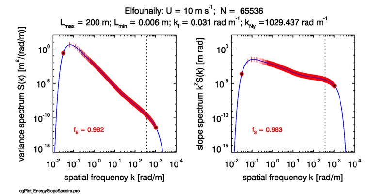
Figure 2 shows the sampling points when . Now the sampled points extend into the capillary-wave spatial scale: the smallest resolvable wave is 0.006 m. (Note that the fundamental frequency is fixed by the choice of , which also fixes the spacing of the samples, .) The elevation variance integral over the sampled ranges is unchanged (we are still missing a small bit of the variance from the very longest waves with frequencies below . However, the slope integral is now . Thus we are now sampling a fraction of the slope variance. The resolution of both the elevation and slope spectra are now acceptable for almost any application. Although using a very large is computationally feasible in one dimension, such a large is computationally impracticable in two dimensions, when we would need a grid of size . In the present example, this would would require of storage for just one real array, as well as a corresponding increase in run time for the FFT. Another approach to resolving the slope variance is therefore needed.
As we have just seen, the unsampled frequencies greater than the Nyquist frequency can account for a large part of the slope variance. These frequencies represent the smallest gravity and capillary waves. The amplitudes of these waves are small, so they contribute little to the total wave variance, but their slopes can be large. One way to account for these “missing” waves is to alias their variance into the waves of the highest frequencies. The highest frequency waves that are sampled will then contain too much variance, i.e., they will have amplitudes that are too large for their wavelengths, which will increase their slopes. One way to do this is as follows.
We seek an adjusted or re-scaled elevation spectrum
| (5) |
such that the integral of over the sampled region equals the integral of the true over the full spectral range. Then sampling the re-scaled spectrum will lead to the same slope variance as would be obtained from sampling the correct spectrum over the entire range of frequencies.
We can choose so that the low frequencies are well sampled starting at the fundamental frequency . There is thus no need to modify the low-frequency part of the variance spectrum, which if done, would adversely affect the total wave variance. We want to modify only the higher frequencies of the sampled region, which contribute the most to the wave slope but little to the wave elevation. A simple approach is to take to be a linear function of between the spectrum peak and the highest sampled frequency , and zero elsewhere:
is a parameter that depends on the spectrum (i.e., the wind speed), the size of the spatial domain, and the number of samples . We must determine the value of so that this “adds back in” the unresolved slope variance. The added variance will be zero at the peak frequency and largest at the Nyquist frequency. That is, the function will make only a small change to the variance spectrum at the low frequencies, and the change will be largest near the highest sampled frequencies, which is consistent with the idea that the high frequency waves have the largest slopes. (There is nothing physical about the functional form of Eq. (6); it is simply a single-parameter ad hoc function that works reasonably well in practice. Nonlinear functions could be used, e.g. to concentrate more of the variance into the frequencies closest to the Nyquist frequency. However, those functions could have more than one free parameter to determine and, in any case, the end result is the same: a sea surface that reproduces the height and slope variances of the fully sampled spectrum.)
To determine we thus have
The right-most terms of these equations give (after recalling that for )
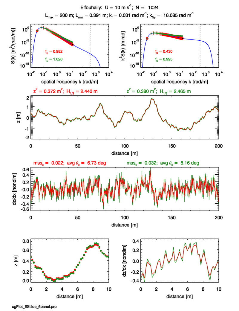
| (7) |
Figure 3 shows example 1-D surface realizations created with samples and both the true and scaled variance spectra. The upper two panels reproduce Fig. 1, except that the sampled points of the re-scaled spectra are shown in green. It is clear that the function has added progressively more variance to the higher frequencies. The re-scaled variance spectrum does of course contain somewhat more elevation variance over the sampled region than does the true spectrum. As the green inset number shows, this re-scaling has increased the fraction of sampled/true variance from 0.982 to 1.020. However, the number in the upper-right panel shows that we are now sampling 99.5% of the slope variance, as opposed to 43% for the true spectrum. Having a bit too much total elevation variance is a good tradeoff for being able to model the optically important slope statistics.
The row 2 panel shows random realizations of the 1-D surfaces generated from these two spectra (with the same set of random numbers). The surface elevations generated using the true spectrum (red line) and the re-scaled spectrum (green line) are almost indistinguishable at the scale of this figure. These significant wave heights for these two surface realizations compare well with the significant wave height of for a Pierson-Moskowitz spectrum. The row 3 panel shows the surface slopes computed from finite differences of the discrete surface heights. The Cox-Munk along-wind mean square slope is given by , which compares well with the value of 0.032 obtained with the re-scaled spectrum. However, the value obtained from the true spectrum is only 0.022, or 70% of the Cox-Munk value. The bottom two panels replot the 0-10 m sections of the and figures for better display of the details.
We thus see that when using the correction to a variance spectrum, we can generate a surface that reproduces, to within a few percent of the theoretical values, both the surface elevation and slope statistics that would be obtained from the underlying true variance spectrum if it were sampled with enough points to fully resolve the elevation and slope variances.
 See comments posted for this page and leave your own.