Page updated:
March 22, 2021
Author: Curtis Mobley
View PDF
Time-Dependent Surfaces
One final step remains: the addition of time dependence to generate a sequence of the sea surface realizations. Many scientific applications do not need time dependence. This is the case when many independent random realizations of sea surfaces are used for Monte Carlo ray tracing to compute the average optical reflectance and transmittance properties of wind-blown sea surfaces. However, time dependence is crucial for applications such as computer-generated imagery for movies.
We already have the needed theory in hand from the page on Spectra to Surfaces: 2D. The fundamental are equations from that page are
and
| (2) |
These quantities are evaluated as described on that page, but with the evaluations done at particular times . Most importantly, these equations make no simplifying assumptions about the symmetry of the two-sided variance spectrum .
As we have learned, the Fourier transform of a snapshot of the sea surface gives a two-sided variance spectrum with identical values for and . This represents equal amounts of energy propagating in the and directions, i.e., equal amounts of energy in waves propagating upwind and downwind. Such a situation in nature gives standing waves. Here also, if , the time-dependent surface will be standing waves composed of waves of equal energy propagating the and directions. To obtain waves propagating downwind, as is the case in a real ocean, we must use an asymmetric two-sided spectrum with , so that almost all of the energy is propagating downwind. Note, however, that we cannot simply set , which represents no energy at all propagating upwind. This is because destroys the Hermitian property of Eq. (2). Thus we must conjure up an asymmetric variance spectrum that allows a nonzero (although perhaps negligible) amount of energy to propagate upwind.
An asymmetric two-sided variance spectrum can be constructed using an asymmetric spreading function as described on the previous page, Spreading Function Effects . Spreading functions of the form
| (3) |
described there allow some energy to propagate in directions, i.e. when . With this choice of a spreading function, we can let the magnitude of equal the magnitude of the one-sided variance function , which gives the total variance, because we assume that a negligible amount of the total energy propagates in directions. With this assumption, there is no division of by 2 in the first line of Eq. (1). That is, we are starting with a two-sided, asymmetric spectrum, not with a one-sided spectrum based on the assumption of upwind-downwind symmetry.
Once an asymmetric has been defined, we can evaluate Eq. (1) for a set of random numbers and . This is done only once. Then to generate a sequence of sea surface realizations for times , we multiply the time-independent amplitudes by the time-dependent cosines and sines as was shown previously in
We thus obtain the amplitudes at the current time . The inverse Fourier transform of this gives the sea surface at time .
The physics (or lack thereof) of this process is simple. We start with a realization of the sea surface at time zero. This surface contains waves of many discrete frequencies traveling in all directions . Then to get the surface at any later time , we simply propagate the sinusoidal waves of each frequency in their original direction of travel through a phase change determined by the time step and the dispersion relation . For deep-water gravity waves, the dispersion relation is . It thus visually appears that the waves are propagating and the sea surface profile is changing with time. However, this Fourier transform technique is really just moving a collection of independent, non-interacting sinusoids through frequency-dependent phase angles to create a new surface realization from the sum of the phase-shifted sinusoids. In a real ocean, waves of difference frequencies can interact with each other (redistribute energy among frequencies) in highly complex and nonlinear ways, so that the sea surface statistics may not be time-independent. This is, in particular, how little waves grow to big waves when the wind begins to blow over a level surface. Modeling the nonlinear evolution of a sea surface is beyond the abilities of Fourier transform techniques which are, at heart, just a mathematical artifice based on a time-independent directional variance density spectrum.
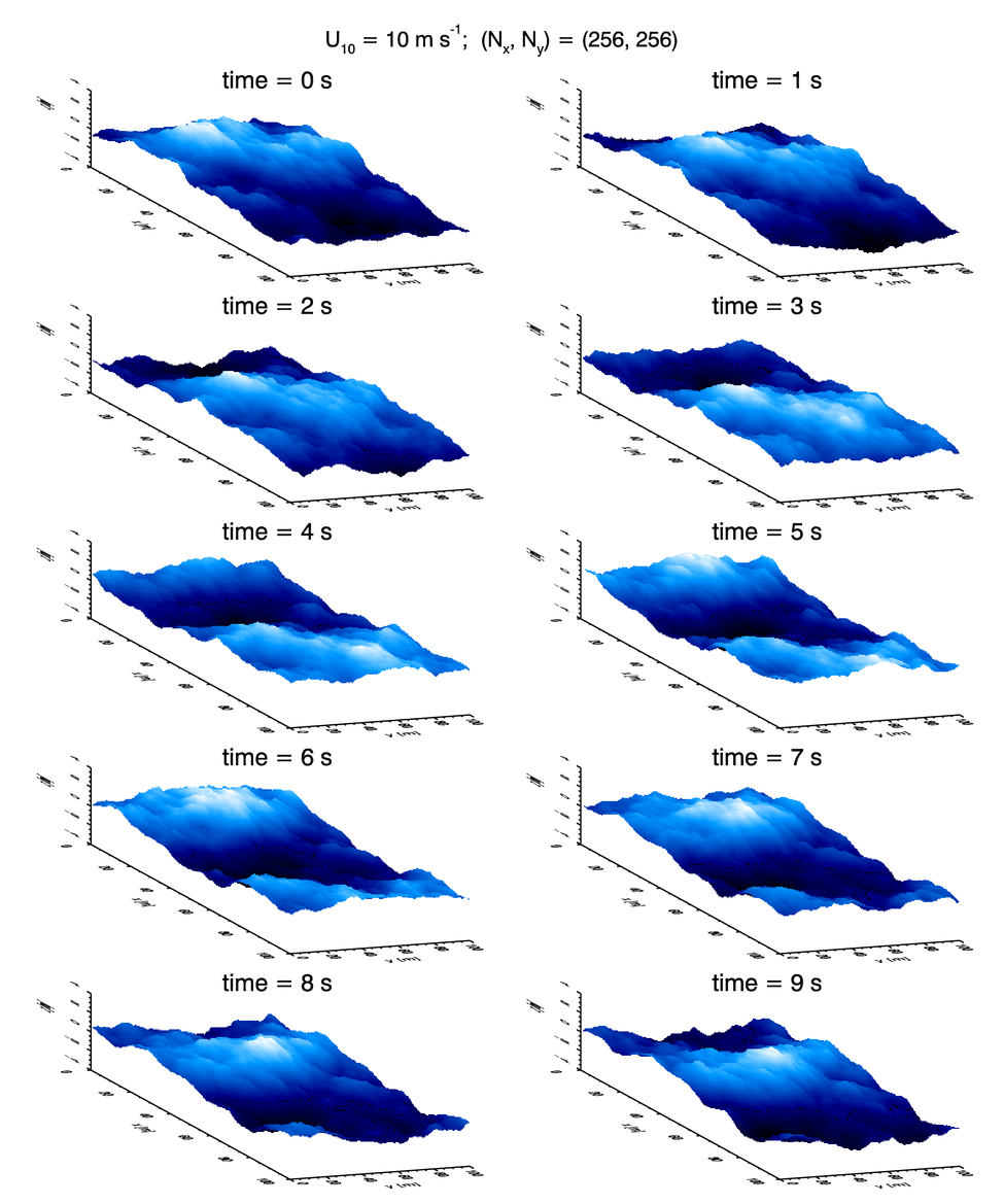
Figure 1 shows a sequence of surface realizations for a wind speed and a spatial grid of size , and a grid resolution of . A time series of images made with such a course grid could be useful for some non-scientific purposes.
We have seen that the spatial pattern of a sea surface generated by a Fourier transform is periodic. This is convenient for tiling a small computed region into a visually acceptable larger region. When time dependence is included and a finite-length time series of images is created, the sequence of images is not periodic in time because the various sinusoids comprising the surface do not have a common period. As pointed out by Tessendorf (2004), this can be remedied by “quantizing” the temporal frequency as follows.
Let be the length of time over which the time sequence of surface realizations should exactly repeat. The number of frames in the video loop determines the time step between frames, . For a smoothly moving sea surface, must be large enough that is less than about 0.1 s. Define . For deep-water gravity waves, the true temporal frequency is replaced by
| (5) |
where converts a real number into its integer part (e.g., 15.23 is converted to 15). This operation slightly alters the temporal frequency of each wave component so that each component returns to exactly its initial shape after time . A video loop can then be created from the sequence of surfaces, and the loop will match perfectly when the frame for time goes to the frame for time , which is the same surface as time 0, after which the surfaces repeat. This adjustment to is greatest for the lowest frequencies, but the adjustment becomes smaller and smaller as the repeat time becomes larger and larger. It is thus easy to create a time-dependent small area of sea surface that can be tiled in both space and time to create an image of a larger sea surface over a longer time. This is good enough to fool movie-goers.
In order to employ a re-scaled variance spectrum as described on page Numerical Resolution, determine the value of the parameter using the omnidirectional variance spectrum, as seen in Eq. (7) of that page. Then apply the correction to the directional spectrum with for each point of the rectangular grid.
An example of a 20-second (simulated time) video loop created using all of these tricks can be seen at video loop. This shows a time series of 2D sea surface realizations generated using the variance spectrum of Elfouhaily et al. (1997) with a frequency-dependent cosine-2S spreading function. This omnidirectional elevation variance spectrum was adjusted as described on page Numerical Resolution at the higher spatial frequencies so that unresolved slope variance (from frequencies higher than the and Nyquist frequencies resolvable by a 512 by 512 DFT grid) is fully resolved. The true dispersion relation was quantized for each discrete spatial frequency so that the surface is exactly periodic after 20 seconds. Note in particular that the significant wave heights are slightly greater on average than the value of 2.25 m predicted by a Pierson-Moskowitz spectrum, which has somewhat less energy than the Elfouhaily et al. spectrum used here. Note also that the along-wind () and cross-wind () mean square slopes are very close to what is expected by Cox-Munk statistics: 0.031 and 0.019 respectively. The sequence of plots used to create the video loop was created by IDL routine cgAnimate_2D_SeaSurface.pro. The plots created by the IDL routine were then combined into the video using VideoMach.
 See comments posted for this page and leave your own.