Page updated:
April 2, 2021
Author: Curtis Mobley
View PDF
Visualizing Radiances
Even in the simplest case of horizontally homogeneous water and time independence, the radiance distribution is a function of four variables: depth , polar angle , azimuthal angle , and wavelength . This makes it hard to display radiances graphically and to understand the wealth of information contained in for given environmental conditions. The following figures show some of the ways commonly used to present radiance distributions. These figures also give us our first chance to study the nature of oceanic radiance distributions.
To obtain a complete radiance distribution for these figures, the HydroLight numerical model was run for very simple conditions:
- a bio-optical model for homogeneous Case 1 water was used with a chlorophyll value of (a typical value for open-ocean water) to generate the absorption and scattering properties of the water
- the sun was placed at a solar zenith angle of 40 deg in a clear sky with typical values for marine atmospheric conditions
- the sea surface was flat (wind speed of 0)
- the water was infinitely deep
- fluorescence by chlorophyll and CDOM, and Raman scatter by water, were included
- radiances were computed on a 10 by 15 deg angular grid; the computed radiances are thus the average radiances over each 10 by 15 degree angular “window”
- radiances were computed at 10 nm wavelength resolution between 350 and 700 nm; computed radiances are thus the averages over 10 nm bands from 350 to 360 nm, etc.
Figure 1 shows how this HydroLight-computed radiance distribution in air just above the sea surface depends on polar viewing direction and wavelength, in the azimuthal plane containing the sun. This figure requires considerable explanation. In HydroLight the polar angle is measured from 0 in the or downward direction to 180 deg in the or upward direction (depths are commonly measured as positive downward in oceanography, and polar angles are commonly measured from the direction). Thus photons heading straight down have a polar angle of . This plot uses the viewing direction , which is the direction an instrument would point when measuring the radiance. Thus the polar viewing angle of means looking straight down (nadir-viewing) and seeing the radiance heading straight up (the upwelling radiance ; i.e., rays traveling upward in the direction). The Sun is located at (solar photons travel in the direction). This figure shows the full range of polar angles in the plane of the sun. The plotting convention is that positive polar angles are looking toward the Sun (the half plane) and negative polar angles are looking away from the sun (the half plane) Thus corresponds to looking horizontally towards the sun, and corresponds to looking horizontally away from the Sun. The range of values between 0 and +90 and between 0 and -90 correspond to looking downward. The range of values from 90 to 180 to -90 on the plot axis correspond to looking upward. The thin black lines show the computational grid. The colors correspond roughly to the visual colors of the various wavelengths. Note that the radiance values are plotted on a logarithmic scale.
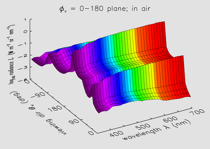
The sun’s radiance is the large spike at , which corresponds to looking upward at a zenith angle of 40 deg in the azimuthal direction, where the sun was located in this simulation. The smaller spike at is the sun’s specular reflection, seen looking downward and towards the sun. The ratio of the sun’s specular reflectance at 355 nm , obtained from the radiance values tabulated in the data file) to the sun’s direct beam is 0.026, which is consistent with the Fresnel reflectance for this incidence angle and water index of refraction (n = 1.34). The broader radiance peak near is the relatively bright near-horizon sky radiance and its reflection by the sea surface, seen looking away from the sun.
Figure 2 shows the radiance in the water at depth 0, i.e. just below the level sea surface. The plotting conventions are the same as for Fig. 1. Note that the large spike of the sun’s direct beam has shifted to a smaller zenith angle near 30 deg (i.e., a larger , now near 150 deg) underwater, in accordance with Snell’s law for refraction across a level air-water surface. The specular reflectance spike in the plot has of course disappeared.
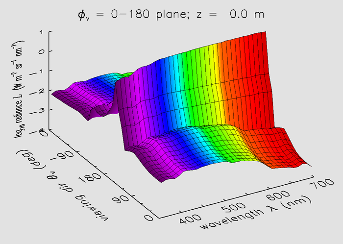
Figure 3 shows the radiance at a depth of 10 m. The radiance distribution is now “smoothing out” because of the effects of scattering, which redirects the original photon directions. However, the direction of the sun’s direct beam is still obvious. The effect of chlorophyll fluorescence on the upwelling radiance near 685 nm is quite obvious as the “bump” in the values near and . The contribution of fluorescence to the downwelling radiance near 685 nm is not as obvious because much of the downwelling radiance is still from sun light that has penetrated to this depth.
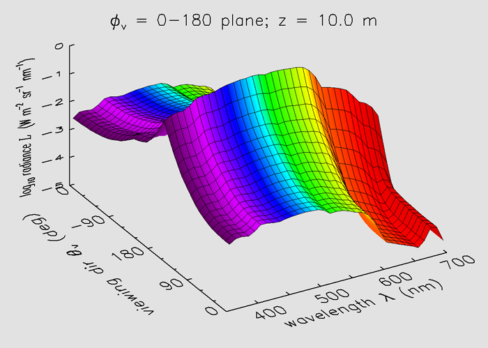
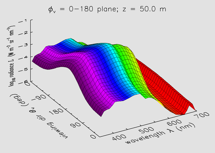
Figure 4 shows the radiance at a depth of 50 m. Now multiple scattering has removed almost all information about the sun’s zenith angle. This radiance is close to the asymptotic radiance distribution, which is determined only by the water’s absorption and scattering properties, and not by the boundary conditions (the solar location in particular) at the sea surface. Chlorophyll fluorescence is now responsible for almost all of the red light near 685 nm in all directions, since the sun’s beam does not penetrate this deep at red wavelengths because of absorption by water.
The information seen in Figs. 1-4 does not show the azimuthal dependence of the radiance, except in the plane containing the sun. Figure 5 illustrates both the polar and azimuthal dependence of the radiance at one depth, in air, and one wavelength, 555 nm. To interpret this plot, imagine that you are at the center of the sphere. The solid black line around the “equator” is looking horizontally . The solid black line drawn from “pole to pole” is the azimuthal direction. The dotted lines show the HydroLight computational grid. The radiances computed as averages over each dotted-line window have been spline interpolated to a 5x5 degree grid for generation of the contours in this figure. Values of of the radiance in are contoured and color-coded for display as a function of and . The colors now represent the magnitude of the , with violet being lowest magnitude and red highest.
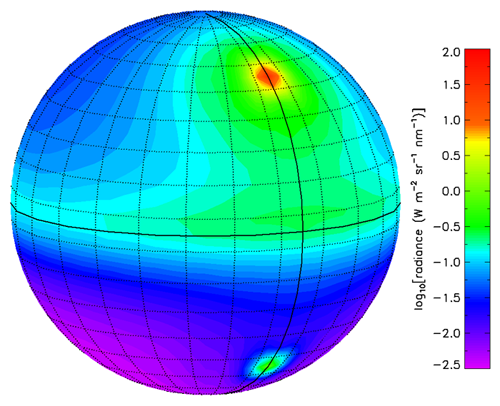
In this figure the “northern hemisphere” represents looking upward toward the sky, and the “southern hemisphere” represents looking downward toward the sea surface. Thus the sun is the red spot seen looking upward at a zenith angle of 40 deg in the direction. (The sun is centered in the computational window that extends from 35 to 45 deg in zenith angle, and in a 15 deg wide window centered on .) The corresponding green spot “below the equator” at is the Sun’s specular reflectance seen looking toward the Sun but downward at a nadir angle of 40 deg.
The detailed directional information seen in Figs. 1-5 is seldom necessary in optical oceanography. It is often sufficient to display the radiance in a few selected directions as a function of depth and wavelength, as in the next two figures.
Figure 6 shows the radiance in five directions: upwelling or nadir-viewing, ; downwelling or zenith-viewing, ; and horizontal directions looking at azimuthal angles toward, at a right angle to, and away from the sun’s azimuthal direction. These radiances are plotted as functions of depth at one wavelength, 555 nm. Although radiances and irradiances are generally thought of as decreasing with depth, this is true only away from the surface. Note that several of these radiances actually increase with depth in the upper few meters of the water column, below which they then decrease. This increase is caused by scattering (path radiance) into the direction being plotted, as the sun’s direct (unscattered) beam is redirected by scattering within the water.
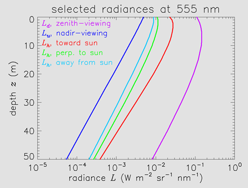
Figure 7 shows the downwelling or zenith-viewing radiance plotted as a function of wavelength for selected depths. The downwelling radiance in air, which is the zenith sky radiance, is plotted in black. The in-water curves are plotted in color using the same wavelength coding as in Figs. 1-3. Note that the downwelling radiance in water at depth is greater than the downwelling radiance in air just above the sea surface. This may seem counterintuitive, since some of the downwelling radiance in air is lost to surface reflection when passing into the water. This increase in when going from air to water is a consequence of the “ law for radiance.” This law, also called “the fundamental theorem of radiometry,” (see Light and Water, p 161) states that the radiance divided by the square of the index of refraction, , remains constant as light travels through regions of different n, to the extent that absorption and scattering can be neglected. Because of Snell’s law of refraction, a given solid angle in air, , becomes in water. Although about 2.6% of the downwelling photons from the sky are Fresnel-reflected back upward for n = 1.34, most enter the water. Those transmitted photons then travel in a smaller solid angle, and thus the associated underwater radiance is greater by a factor of roughly . Some of the downwelling radiance at z = 0 is also due to upwelling radiance being reflected back downward by the sea surface, but this contribution to is small since is typically one to two orders of magnitude less than . Note that at 10 m is greater than the vaules a z = 0 for blue to green wavelengths. This is the same behavior as was seen at 555 nm in Fig. 6.
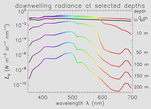
By 200 m depth the blue-green downwelling radiance has decreased by 5 orders of magnitude from the surface value, and other wavelengths have decreased even more. The dominant wavelength is near 500 nm. To get a rough feeling for how this would appear visually, assume that the radiance distribution is isotropic and of magnitude over the 50 nm band from 475 to 525 nm, with other wavelengths being negligible. The corresponding plane irradiance is then . As seen in the Light from the Sun discussion, this is comparable to a moonlit night. Thus the available light at 200 m in this simulated ocean would appear as a very faint bluish green. This is reminiscent of what explorer William Beebe reported during his pioneering bathysphere dives in the 1930’s. In one dive near Bermuda (in water that was likely lower in chlorophyll than the 0.5 used here, hence bluer and more transparent) he reported (Beebe, 1934)
“The green faded imperceptibly as we went down, and at 200 feet [61 m] it was impossible to say whether the water was greenish-blue or bluish-green....At 600 feet [183 m] the color appeared to be a dark, luminous blue, and this contradiction shows the difficulty of description. As in former dives, it seemed bright, but was so lacking in actual power that it was useless for reading and writing.”
If you wish to explore this radiance distribution more, you can download the data file and the IDL plot programs used to create the figures above.
 See comments posted for this page and leave your own.