Page updated:
October 13, 2021
Author: Curtis Mobley
View PDF
Maxwell's Equations in Matter
This page considers electric and magnetic fields inside materials.
Dielectrics
We begin with the effects of electric fields on dielectrics. Dielectrics are materials that do not easily allow the flow of electric charge, so they are also called insulators. Dielectrics include materials like water, glass, wood, or plastic, but not metals, which easily conduct electricity.
The molecules making up many dielectrics have the center of the negative electric charge (due to the electrons surrounding the nuclei) offset slightly from the center of the positive charge (due to the protons in the nuclei). Such molecules are called polar molecules. (The molecule overall is of course electrically neutral.) This offset gives the molecule a dipole moment whose magnitude is defined as the product of the positive charge times the distance between the charge centers. By convention, the direction of the dipole moment vector points from the negative to the positive charge. For example, in the asymmetric water molecule, the electrons tend to cluster around the oxygen atom, leaving the center of the positive charge a bit toward the point between the two hydrogen atoms. A water molecule has a dipole moment of about .
For macroscopic volumes of matter, the combined effect of the molecular dipole moments is described by the net dipole moment per unit volume , which is called the polarization and has units of . (Note that this use of the term “polarization” has nothing to do with the polarization of light.) If the molecules are randomly oriented as illustrated in Fig. 1(a), the molecular dipole moments in the difference directions cancel out so that the net dipole moment of the substance is zero.
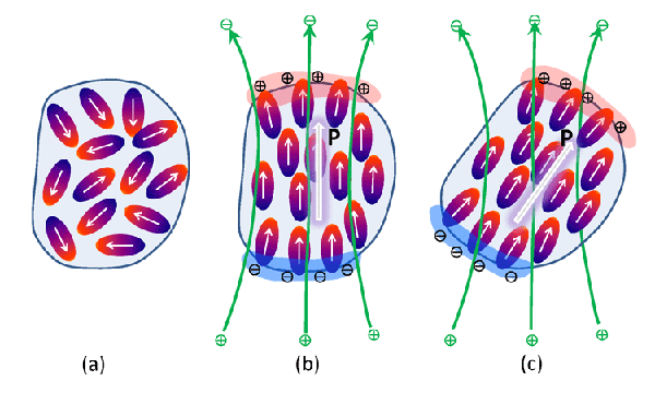
However, if the dielectric is placed in an external electric field, that field can cause the dipole moments to align so that the substance has a net dipole moment, or non-zero polarization , as illustrated in Fig 1(b). In this figure, the green symbols with plus and minus signs represent positive and negative charges creating the external electric field, which is illustrated by the green arrows. The negative ends of the polar molecules are attracted to the positive charges creating the external field, and the positive ends to the negative external charges, so the molecules align as shown. (In practice, this is a complicated business. The applied electric field tends to align the polar molecules, but random thermal motions tend to randomize the directions. Thus, for a given material, depends on temperature. It takes time for the molecules to rotate into alignment, so if the applied field is not constant, depends on the frequency of the applied field. These details need not concern us here, but this is the origin of the frequency (wavelength) dependence of the index of refraction, for example.)
Note that as the molecules align in response to the external field, there is a net accumulation of positive charge on the surface of the material nearest the negative external charges, as illustrated in Fig 1(b) by the reddish area and the black symbols with plus signs. In essence, the positive “heads” of the molecules are sticking out of the volume of material. Likewise, there is an accumulation of negative charge on the opposite side of the material caused by the negative “tails” of the molecules, as illustrated by the bluish area and the black symbols with minus signs. In the interior of the matter, the net charge remains zero because nearby positive heads and negative tails cancel each other out. The external charges (the green + and - symbols in Fig. 1(b)) creating the applied field are called “free” charges because I am free to place them as desired in order to create the external electric field. The charges on the surface of the material are called “bound” charges because they are fixed to the material and cannot be moved around as desired.
The bound charges on the surface of the material create an electric field directed opposite to the applied field. Recall the bookkeeping: electric fields are by convention directed from positive to negative charges, but dipole moments, hence , are directed from negative to positive charges. Thus we expect that the total electric field inside the material will be less than the externally applied electric field. This is why capacitors are filled with dielectric material. By decreasing the electric field between the plates of the capacitor, the capacitor can store more charge before a spark jumps from one plate to the other. The field set up by the bound charges will also distort the field of the free charges in the region outside the dielectric.
Even if the molecules or atoms of the dielectric are symmetric and have no dipole moment in the absence of an electric field, they will become polarized in the presence of an applied field. This is because the applied field tends to pulls the negative electron cloud in one direction and the positive nucleus in the other direction, creating a dipole moment.
The situation just discussed is called induced polarization, because the polarization is induced by the applied external electric field. The direction of the polarization vector is then parallel to the applied field . This is not always the case. Some crystals have a permanent polarization due to their molecular structure. These substances are called “electrets” and are the electrical equivalent of permanent bar magnets. (Indeed, the name comes from“electric magnets”.) Examples are quartz crystals and barium titanate, . In this case, illustrated in Fig. 1(c), the polarization is not induced by the applied field and can be in any direction relative to the applied field.
Maxwell’s Equations in Matter
To continue the development, recall for reference the forms of Maxwell’s equations in vacuo:
The total electric field is equal to the field of the free charges plus the field of the bound charges. In practice, we control the free charges and can place them as desired, but not the bound charges, which are stuck to the material. In the most general case, there may even be bound charges induced within the material if the material is inhomogeneous so that varies with location. A general expression for the bound charge density is then (e.g., Griffiths (1981), Section 4.2)
We can now write the total charge density as the sum of the free charge density and the bound charge denisty:
Inserting this into Eq. (1) gives
Defining the electric displacement as
| (5) |
allows Eq. (1) to be rewritten as
| (6) |
The significance of this development warrants discussion. In Gauss’s law, , the charge density includes all charges, both free and bound (if any), and the electric field is the total electric field caused by all charge density. This is the electric field either outside or inside a dielectric. It is that we normally want to know. Although we can define the free charge density as desired, we may not know what the bound charge density is because that depends on the dielectric material. Determining for a given material and applied electric field can be very difficult (this is what solid state physicists get paid to do). However, we can compute the displacement field given only the free charge density , which we do know, without any knowledge of the nature of the dielectric material or its bound charge density. This gives us something to start with, using only what we know. Then, if we can determine the polarization (which may or may not be easy), we can obtain the electric field from Eq. (5).
In summary, we can avoid having to know the details of the dielectric properties by solving for something, the displacement field, that is not really what we want, but which is related to the electric field. Note that the displacement does not have the same units as , and may not even be in the same direction as (the situation of Fig. 1(c)). (There are other subtleties associated with . For example, there is no equivalent of Coulomb’s law for , but those discussions are left to the textbooks.) Note also that the remaining three Maxwell’s equations (2)-(4) remain unchanged because they do not involve the charge density.
We can repeat the above process for conducting materials such as metals. Now, instead of molecules or atoms having electric dipole moments, either inherent or induced, we consider molecules or atoms having magnetic dipole moments . Magnetic dipole moments are generated by current loops enclosing some area and have units of . The small electric dipoles shown in Fig 1 are now replaced by small current loops, and instead of bound charges we have bound currents. The sum of these magnetic dipole moments is expressed by the magnetization , which is the magnetic dipole moment per unit volume, with units of . As was seen above, the induced electrical polarization aligns with the applied electric field. However, the induced magnetization can align either with the applied magnetic field (paramagenetic materials) or opposite the applied field (diamagnetic materials). Materials with permanent magnetization are called ferromagnetic (an example is a common bar magnet).
The Ampere’s law part of (4) shows how currents generate magnetic fields.
| (7) |
Here the current density refers to all currents, and is the magnetic field either outside or inside matter. In addition to free currents and bound currents , in analogy with free and bound charges, there will also be a current associated with a time-dependent polarization. A change in the electrical polarization of a material implies moving charges around, which gives a “polarization” current . We can thus partition the total current density into three parts:
The bound currents can be either on the surface on an object, or within the object if the magnetization is non uniform. In general (e.g., Griffiths (1981), Section 6.2) the bound current and magnetization are related by
The polarization current is given by
The Ampere-Maxwell law (4) can now be rewritten as
Defining the magnetic intensity by
| (8) |
and recalling the definition (5) of then gives
In this equation, we have hidden our ignorance about the magnetic properties of the material inside the term. Note that the magnetic intensity does not have the same units as the magnetic field , and in general the two are not even in the same direction. However, we can solve for given only the free current density and the displacement , which depends only on the free charge density . Then, if we are smart enough to figure out for the material at hand, we can extract the desired from Eq. (8).
We now have Maxwell’s equations in the form usually seen in discussions of arbitrary materials:
These equations are sometimes called the “macroscopic” Maxwell equations, because they hold inside and outside of macroscopic amounts of matter large enough for the spatial averages underlying and to be defined. The original equations (1)-(4) are then called the “microscopic” Maxwell equations because they hold at even the smallest spatial scales, even between the atoms within materials.
It may seem that we now have four equations in four unknowns, but Eqns. (5) and (8) make clear that all we have done is rewrite the original four equations with their two unknowns. In order to solve these equations, we must specify the free charge density and the free current density along with boundary conditions on the fields.
Comments on Terminology
A word of warning is needed regarding terms and units for magnetic fields. I grew up with called the magnetic field and the magnetic intensity, and I’m too old to change. However, the venerable Jackson (1962), the standard graduate-level text on electromagnetic theory for over 60 years, calls the magnetic field and the magnetic induction. The equally competent and respected Griffiths (1981) calls the magnetic field and the auxillary field. Griffiths (page 232) says calling the magnetic induction is “an absurd choice” because it leads to confusion with electromagnetic induction, which is something totally different. He also says, “ has no sensible name; just call it ’’ ”. The great Arnold Sommerfeld, doctoral or postdoctoral adviser to seven students who later won Nobel prizes, says that (in Electrodynamics, 1952, page 45) “The unhappy term ’magnetic field’ for should be avoided as far as possible.” The thing to keep in mind is that and are the fundamental quantities; and arise from rewriting the fundamental equations (Eqs. 1 to 4 of the previous page) in forms convenient for material media. To make matters even worse, the units of and , whatever you call them, depend on the system of fundamental units chosen. Here I have used SI units (previously called “rationalized mks” units). and then have different units, as we have seen. However, in the cgs (centimeter-gram-second) system, is defined by , where is the speed of light. This is convenient because and then have the same units of Tesla, but then Maxwell’s equations are slightly different. In cgs, the Ampere-Maxwell equation (12) reads . This whole business is a confusing mess; see the discussion in Feynman et al. (1964) §36-2.
This qualitative discussion is sufficient for most oceanographers. If nothing else, you can now hold your own at a cocktail party full of undergraduate physics majors. But in all seriousness, it is worth keeping in mind the importance of Maxwell’s synthesis. He tied together apparently unrelated results describing electric and magnetic fields, finished off Ampere’s law, and showed that light of any frequency is a propagating electromagnetic wave. Everything in the modern world that has to do with electricity or magnetism or optics rests upon these equations—generation of electrical current in a hydroelectric plant, the use of that current in an electric motor, radio, television, mobile phones, computers, microwave ovens, lasers, and so on ad infinitum. In oceanography, the well known Fresnel equations for the reflection and transmission of light at the sea surface arises from solving Eqs. (9)-(12) for a plane wave incident onto an interface between two dielectric media. The widely used Mie theory for the scattering of light by spherical particles is the solution of these equations for a plane wave incident onto a spherical dielectric.
You would have to return to the early 1800s—when lighting was by candles and oil lamps, communication was by handwritten letters delivered by riders on horses, and calculations were done with a quill pen and paper—to live in a world without applications of Maxwell’s equations.
In addition to his work on electromagnetism, Maxwell made major contributions to thermodynamics (the Maxwell relations connecting temperature, entropy, pressure, and volume) and statistical mechanics (the Maxwell-Boltzmann distribution). He developed an explanation for the dynamics of Saturn’s rings that is still used today. He even made the first color photographs. Although less known to the general public, Maxwell stands with Newton, Einstein, and Darwin as one of the most profound intellects the world has ever known.
 See comments posted for this page and leave your own.