Page updated:
March 21, 2021
Author: Curtis Mobley
View PDF
Wave Representations
This page first defines the sinusoidal functions that can be used to decompose waves on the sea surface into sums of sines and cosines. Sampling of sea surfaces at a finite number of points is then discussed.
Sinusoidal Wave Representations
The sea surface can be described using a Cartesian coordinate system. Let be a unit vector chosen to point in the downwind direction, and let be directed upward (from the water to the air) normal to the mean sea surface at . Then is in the cross-wind direction. is the surface elevation in meters at spatial location and time .
Fourier proved in the early 1800’s that, under very general mathematical conditions, an arbitrary function can be written as a sum of sines and cosines of different amplitudes and wavelengths. The sea surface elevation is usually such a function. An exception is a sea surface with waves curling over and breaking on a beach. There can then be multiple air-water surfaces for a given : the point on the surface that sees the full sky, the point above a surfer’s head as the wave curls over her, and the point on the water that supports the surf board. However, for a sea surface without breaking waves, there is only one air-water surface for a given location and time, which can be described as a sum of sinusoids.
The terms and notation needed to describe propagating sinusoidal waves are defined as follows:
- is the amplitude (in units of meters) of the wave. This is one-half the distance from the trough to the crest of a sinusoidal wave. Oceanographers often talk about the wave height, , which is the distance from a wave trough to a wave crest. Wave height is what most people visualize when they talk about how “big” a wave is. For a sinusoidal wave, .
- is the temporal period (seconds), usually called just the period. This is the time it takes for one wave crest to pass by a fixed point, i.e. for the argument of a sinusoid to go through radians.
- is the temporal frequency (1/seconds), usually called just the frequency. This is how many waves pass by a fixed point per second.
- is the angular frequency (radians/second). This is the number of waves passing a fixed point in seconds.
- is the wavelength, or spatial period, (meters). This is the distance from one wave crest to the next.
- is the wavenumber or spatial frequency (1/meters). This is the number of wavelengths per meter.
- is the angular wavenumber or angular spatial frequency (radians/meter). This is the number of wavelengths in meters.
- is the phase (nondimensional). This fixes the location of a wave crest relative to the origin of a coordinate system.
There is no uniformity in the literature. People often refer to “the frequency” without specifying whether they mean or , and “wavenumber” or “spatial frequency” may mean either or . People use , or for the wavenumber, some use for , and so on. You just have to figure it out on a case by case basis. For pedagogic purposes, we will start with wavenumber as the measure of spatial frequency, and then switch to the more common angular spatial frequency . This presentation will use as the measure of temporal frequency.
Now consider a one-dimensional sea surface with elevation over a spatial region of length , e.g. or . According to Fourier, can be written as a sum of sinusoids, the one of which is
| (1) |
where is simply an index for which sinusoid is being considered. (Note that we could just as well write a sine here, which corresponds to a different value for the phase.) For this reduces to a constant offset , which is usually taken to be mean sea level and set to a reference value of 0 via setting . For the moment, take , i.e., we have a snapshot of the ocean surface at time zero. This sinusoid has a wavelength of , i.e., the cosine returns to the same value after a distance of . It is a pure cosine in the chosen coordinate system if the phase is or an even integer multiple of . If the phase is an odd integer multiple of it is a sine. If time is included, the wave is propagating in the direction if the time term is ; the cosine returns to its initial value after a time of . A wave propagating in the direction is described by a term. The physical angular frequency is always positive, but mathematically we can write just in the equation and then view a wave propagating in the direction as having a negative temporal frequency.
With this interpretation of , Eq. 1 is conveniently written as
| (2) |
where is the angular wavenumber of the wave of wavelength . Likewise, is the angular frequency of the wave with period . It may be intuitively easier to think of wavelengths per meter than of wavelengths per meters, but the convenience of writing rather than or makes rather than the spatial frequency variable used in most publications. A similar comment holds for vs. , so rather than is the common choice for the temporal frequency variable.
If we take , or just combine the time term with the phase, expanding the cosine in Eq. (2) gives an equivalent form
| (3) |
where and , and . This equation can be written in terms of complex numbers:
| (4) |
where and
| (5) |
Recalling that , we see that the imaginary parts of Eq. (4) add to zero, so that is still a real variable even though it is written in complex form. Also note that , where denotes the complex conjugate. (Complex conjugation means replace by in all terms.) Although two complex numbers in general contain four independent real numbers, these and pairs contain only two independent numbers, and .
We thus have three ways to describe a sinusoidal wave: (1) The cosine of Eq. (2) defined by an amplitude and a phase; (2) the cosine and sine of Eq. (3) defined by two amplitudes, or (3) the complex exponentials of Eq. (4) defined by two complex numbers containing two independent real numbers. These equations all give the same , so we are free to choose whichever form is mathematically convenient for the problem at hand. For visualization of sea surfaces, the real forms (2) or (3) are convenient, but the calculations on the next pages are most conveniently carried out using complex exponentials.
Returning now to Fourier, linear wave theory says that we can write the sea surface elevation as a Fourier series
| (6) |
which in conjunction with Eq. (4) can be rewritten as
| (7) |
As previously noted, the or term is usually set to 0. This equation is the mathematical heart of our subsequent descriptions sea surfaces.
Although the physics that leads to a given sea surface in general involves non-linear interactions between waves of different wavelengths and periods, the shape of the resulting sea surface can be written as a linear sum of sinusoids of different frequencies. Owing to the orthogonality of sines and cosines for different values as defined above, these wave components are independent of each other. (Orthogonality means that if , etc.) Thus a description of a time-dependent surface based on an expansion like that of Eq. (6) (including the time-dependent terms as seen in Eq. (2)) cannot be used to predict the nonlinear evolution of a sea surface from a given initial condition. To do that, you must return to the world of hydrodynamics in all of its nonlinear glory. For our present purposes, we only want to model the shapes of sea surfaces, not predict their hydrodynamic development from an initial state, so linear wave representations are adequate.
Sampling
We next consider the implications of sampling the sea surface at a finite number of discrete locations or times. It is usually the case when we want to measure the sea surface elevation that we either make measurements at discrete locations at a given time, or at discrete times at a given location.
For a specific example, consider a region of sea surface long where we take evenly spaced samples. This gives a measurement every at a given time. We are going to describe this surface as a sum of sinusoids. Figure 1 illustrates the first few sinusoids shown as cosines. The cosines in the figure all have the same amplitude and each is offset vertically for ease of viewing. The dots show the sampled values for each cosine component.
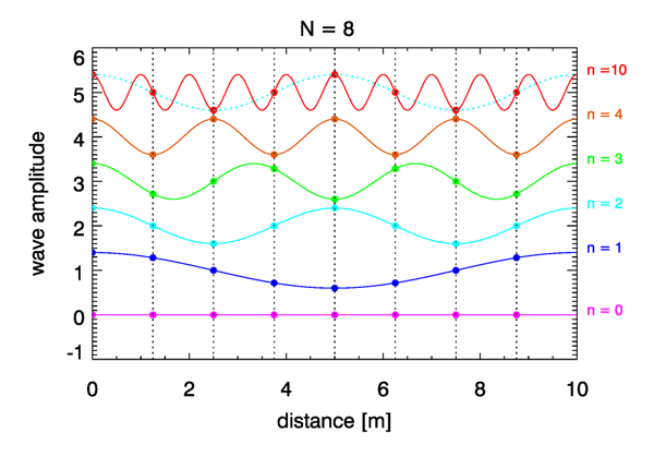
The longest wave that can fit into a region of length has a wavelength of . This is called the fundamental wave or first harmonic. This wave is shown by the blue curve in the figure. Note that the cosine in the figure has a period of . The smallest wave that can be captured correctly in a sampling scheme has a period of twice the sampling interval. This called the two-point wave or two-point oscillation. Note that a sine term with period would be sampled at arguments of where the sine is zero and is thus not detectable. The spatial frequency (or temporal frequency if sampling in time at a given location) is called the spatial (or temporal) Nyquist frequency. Waves with higher frequencies than the Nyquist frequency are still sampled, as illustrated by the dots on the wave with . Note, however, that the pattern of sampled points for the wave is exactly the same as for the wave. If all we have are the measured points, we cannot distinguish between the and the waves in this example. This illustrates the phenomenon of aliasing. In general, a wave with a frequency greater than the Nyquist frequency (i.e., a wavelength or period less that twice the sampling interval) is still sampled, but it appears as though the high frequency wave is a wave with a frequency less than the Nyquist frequency. The information about the high frequency (short wavelength) wave is added to or aliased into a lower frequency (longer wavelength) wave, thereby giving incorrect information about the lower frequency wave. Aliasing places a severe constraint on any sampling scheme. We can correctly sample only waves with wavelengths that lie between the size of the spatial region, , and twice the size of the sampling interval. (In the temporal setting, the limits are the length of sampling time and twice the temporal sampling interval.)
The relation between a sampled frequency greater than the Nyquist frequency, the sampling rate or Nyquist frequency , and the frequency receiving the aliased signal is
where is the closest integer multiple of the sampling rate to the signal being sampled. In the example of Fig. 1, , , and either or gives (or ). Thus the wave is aliased into the wave, which has a frequency of 2 waves per 10 meters, or , just as seen in the figure. Note that many other frequencies are also aliased into this frequency. For example, a wave with , corresponding to , also gives = 0.2 with , and so on.
 See comments posted for this page and leave your own.