Page updated:
May 23, 2021
Author: Curtis Mobley
View PDF
Surfaces to Spectra: 1D
This page uses a contrived example to illustrate the preceding theory for a one-dimensional (1D) surface. Detailed comments on this simple example emphasize the mathematical subtleties and physical characteristics of Fourier transforms and wave variance spectra derived from surface elevations. A thorough understanding of this example takes us much of the way to understanding the case of a real ocean surface.
An ad hoc, one-dimensional wave profile is constructed using the formula
| (1) |
The locations are given by , where is the length of the sea surface region being sampled and is the number of samples. is the fundamental spatial frequency, that is, the spatial frequency or wavenumber of the wave with a wavelength of . The amplitude of the wave at the frequency, , is chosen to be
and . The phase of the wave component is randomly distributed over using
where is a uniform random number. A different random number is drawn for each value.
The upper left panel of Fig. 1 shows the surface generated in this manner for , , and a particular set of random phases. Note that is a power of 2 as will be needed for the FFT. The thin colored lines show the waves for each of the frequencies. The blue line is the wave for the fundamental frequency ; the thin black line is the two-point wave at the Nyquist frequency ; the purple line is the constant wave, which is set to for the mean sea surface. The black dots connected by the thick black line show the sum of the individual waves. These points represent a discrete sampling of the continuous sea surface elevation.
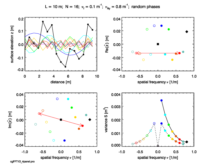
In this example, the sampled region of the sea surface is in length, but the samples do not include the point at . This is because the surface elevation at is always the same as at when using Fourier techniques. Resolving the surface as a sum of sinusoids that are harmonics of the fundamental frequency gives sinusoids that always return to their initial value after distance . Real sea surfaces are of course not periodic, but we do not know the true value at because it was not measured by the present sampling scheme. (Likewise, we do not know the true surface elevations at points in between the sampled locations.) When we use Fourier techniques to generate random surface realization, we are always generating a sea surface that is a periodic tiling; the tile dimension is . This periodicity is useful if we want to generate a visual rendering of a large region of sea surface from a smaller computed region; the edges of the small tiles will match perfectly and the larger surface will often look reasonable, if you don’t look too closely. An example of a tiled two-dimensional surface can be seen in Fig. 3.9 of Mobley (2016).
We now take the sequence of the real wave elevations seen in Fig. 1 and feed them into an FFT routine. We soon get back 16 complex numbers, the Fourier amplitudes, at a set of 16 corresponding frequencies . The upper right panel of Fig. 1 plots the real part of the complex numbers, and the lower-left panel plots the imaginary part.
Note first that the FFT routine returned both negative and positive spatial frequencies:
for a total of discrete spatial frequencies. Note that the frequency spacing equals the fundamental frequency . The Fourier Transforms page discussed the interpretation of negative frequencies. (The order of the frequencies as returned by the FFT routine was the “FFT order” discussed on the Fourier Transforms page. The frequencies, and the corresponding amplitudes, were reordered to get the “math order” used for plotting.)
Note next that the real parts of the complex amplitudes are even functions of frequency: . The imaginary parts are odd functions of frequency: . In Fig. 1 the positive and negative frequencies are connected by a red arrow for one particular frequency pair, . If a complex function has an even real part and an odd imaginary part , then , i.e. the function is Hermitian. Thus the plots verify that the amplitudes are Hermitian, as is always the case for the Fourier transform of a real function. The Hermitian character of the complex amplitudes means that these complex numbers contain only 16 independent real and imaginary numbers, not 32 as would be the case for 16 arbitrary complex numbers. In general the FFT of real numbers (e.g., spatial samples of a sea surface) gives back independent numbers, so that the “information content” of the physical and Fourier representations is the same.
The positive frequency at is the Nyquist frequency. There is, however, no value for the negative of the Nyquist frequency. Note also in the lower left panel that the imaginary part of the amplitude is identically zero at the Nyquist frequency. We will explain these values below.
The lower-right panel of the figure shows the values of . The values at the negative to positive frequencies are connected by the black dotted line. These points constitute the two-sided discrete variance spectrum,
| (2) |
“Two-sided”, denoted by the subscript 2S, refers to spectra showing both the negative and positive frequencies. The variance at zero frequency is the variance contained in the constant mean sea level. This value is zero because we have set the mean sea level to zero.
Oceanographers are often concerned only with the variance at a given magnitude of the spatial frequency, and not with whether the frequency is negative or positive. Nor is there any reason to plot the point at zero frequency, which is usually zero by choice of zero for the mean sea level. It is therefore customary to define the one-sided variance spectrum
| (3) |
for , and . Then only the positive frequencies are plotted. The points connected by the solid black line in the lower-right panel of Fig. 1 comprise the one-sided variance spectrum. In the present simulation, the two-sided spectrum is symmetric for positive and negative frequencies (except for the Nyquist frequency, which does not have a negative counterpart and is always a special case), and the one-sided function is simply twice the value of the two-sided function for the positive frequencies, except for the Nyquist frequency. When you read a paper and it refers to or plots “the variance (or energy or power) spectrum” without further comment, it is always the one-sided spectrum. However, on the next pages we will have to use two-sided spectra, in which case we will have to account for the magnitude difference in one- and two-sided spectra.
There is an important detail to note in the computation and plotting of , as in the lower-right panel of Fig. 1. The values of were obtained by the discrete Fourier transform of Eq. (??), and gives the variance contained in a finite frequency interval at the discrete frequency . equals the fundamental frequency and is the frequency interval used in the calculations and the plot. As noted in the discussion of the discrete transform, is a point function. As was seen in Eq. (13) of the Fourier Transforms page, if we wish to convert the discrete to an estimate of the continuous variance spectral density , we must divide by the discrete function by the frequency interval: . The units of are then , as expected for a spectral density function of spatial frequency. It is important to distinguish between a discrete variance point function and a continuous variance spectral density.
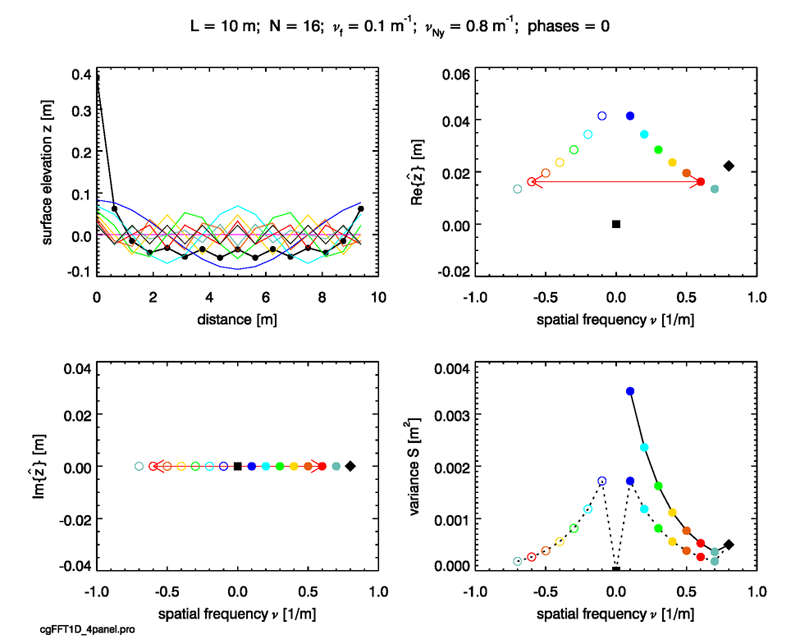
Now return to Eq. (1) and set all of the phases to zero. We are then adding together cosines to create the surface wave profile, which is seen in the upper left panel of Fig. 2. The FFT of this profile gives the real part of as positive numbers except for the 0 frequency, and the imaginary part is identically zero for all frequencies.
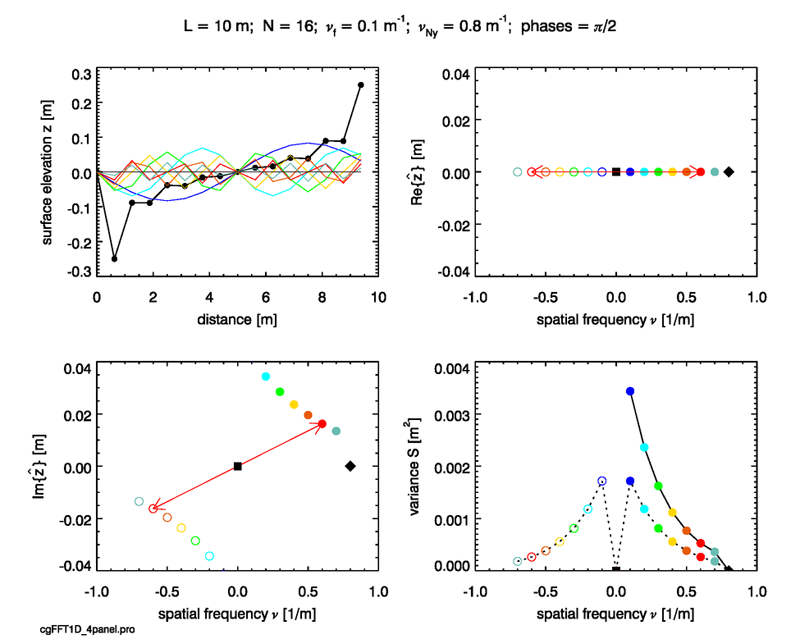
If we set all of the phases to , we are then adding together sines to create the surface wave profile, which is seen in the upper left panel of Fig. 3. The FFT of this profile gives the real part of identically zero and the imaginary part is nonzero except for the 0 and Nyquist frequencies.
These two figures show that the real part of the complex amplitude tells us how much of is composed of cosine waves, and the imaginary part shows how much of is composed of sine waves. This explains why the imaginary part of the amplitude is zero at the Nyquist frequency. The two-point wave at the Nyquist frequency is inherently a cosine wave because, as noted previously, a two-point sine wave is sampled only at its zero values. The general case of a wave component with a phase that is neither 0 (nor a multiple of ) nor (nor an odd integer multiple of ) can be written as a sum of cosine and sine waves, as in Eqs. (3) and (6) of the Wave Representations page. In that case, both the real and imaginary parts of the amplitudes are nonzero (except for the special cases of the 0 and Nyquist frequencies).
Note that in each of these three simulations, which differ only by the phases of the component sinusoidal waves, the variance spectrum is exactly the same (except at the Nyquist frequency), as seen in the lower right panels of Figs. 1-3. That is to say, the variance contained in a wave does not depend on the reference coordinate system used to describe it, even though the Fourier amplitudes do depend on the coordinate system. The variance depends only on the amplitude of the wave. The variance at the Nyquist frequency is largest when cosine waves are added and is zero when sine waves are added. In the first case, we have the maximum possible amplitude of the two-point cosine wave, and in the latter case there is no two-point wave.
 See comments posted for this page and leave your own.