Page updated:
May 23, 2021
Author: Curtis Mobley
View PDF
Spectra to Surfaces: 2D
Now, again, we face the reverse process: start with a two-dimensional, one-sided variance density spectrum and generate a random 2-D realization of a sea surface. The first task is to conjure up a two-dimensional variance density spectrum, which requires some effort.
Theory
Let denote a 2-D elevation variance spectrum as defined on the Wave Variance Spectra: Theory page. This spectrum has units of . By definition, the integral of over all frequencies gives the elevation variance:
As in the 1-D case on page Spectra to Surfaces: 1D, indicates expectation or ensemble average over many measurements of the sea surface.
In the discrete case, the values coming out of point both “downwind” (positive values) and “upwind” (negative values), i.e. there are both positive and negative frequencies represented in the “two-sided” variance spectrum, denoted as as above. In general, because more energy propagates downwind than upwind at a given frequency. is the Nyquist frequency for waves propagating in the direction; is the Nyquist frequency for waves propagating in the direction. is the variance at zero frequencies, i.e., the variance of the mean sea surface; this term is normally set to 0 so that the mean sea surface is at height 0.
The 2-D equivalents of Eqs. (1) and (2) on page Spectra to Surfaces: 1D are
Here, as before, and are independent random variables, with a different random variable drawn for each value. As in the 1-D case, the expected value of gives back whatever variance spectrum is used for , but is not Hermitian. As before, the notation in these equations distinguishes between the value of the continuous spectral density function evaluated at a discrete frequency value, , and the discrete variance point function, .
We must define random Hermitian amplitudes for use in the inverse Fourier transform. Looking ahead to the page on Time Dependent Surfaces, which extends the results of this page to time-dependent surfaces, define the time-dependent spectral amplitude
| (3) |
This function is clearly Hermitian, so the inverse DFT applied to will give a real-valued . Recall that a function of the form gives a wave propagating in the direction. The corresponding in this equation gives a wave propagating in the direction, which is in the downwind half plane of all directions. In general the temporal angular frequency is a function of the spatial frequency . For example, for deep-water gravity waves, .
For simplicity of notation, let us momentarily drop the and subscripts on the discrete variables. The of Eq. (3) is also consistent with the variance spectrum:
Here we have noted that all terms like are zero because of the independence of the random variables for different values, as are terms like . The remaining term is the total variance associated with waves propagating in the downwind and upwind directions at the spatial frequency of magnitude . It should be noted that this term is independent of time even though the waves depend on time. This is because the total variance (or energy) of the wave field is the same at all times, even though the exact shape of the sea surface varies with time.
If only a “snapshot” of the sea surface at one time is available, it is not possible to resolve how much of the total variance is associated with waves propagating in direction compared to the opposite direction . The forward DFT, , and then gives , in which case the last equation reduces to
In any case, the amplitudes defined by Eq. (3) are Hermitian, so that the real part of the inverse Fourier transform gives a real-valued sea surface . That sea surface is consistent with the variance spectrum at every time . Wave variance (energy) is thus conserved in a round-trip calculation from variance spectrum to sea surface and back to variance spectrum. In the time-dependent case, if , then more variance will be contained in waves propagating in the direction than in the direction. This is all that we can ask from Fourier transform techniques.
Although Eqs. (2) and (3) are compact representations of the random spectral amplitudes, the actual evaluation of these equations in a computer program warrants further examination. In particular, the Nyquist frequencies are always special cases because there is only a positive Nyquist frequency, at array element , with a corresponding equation for the Nyquist frequency in the direction. Writing and expanding Eq. (3) gives
These terms are all arrays, but note that terms like represent element-by-element multiplications, not matrix multiplications.
For a particular array element , and using the indexing relation for frequencies written in math order, we can write
This equation allows for efficient computation within loops over array elements. In particular, the code can loop over the non-positive values, , and over all values, to evaluate the amplitudes for all non-Nyquist frequencies. The positive values are then obtained from the negative values by Hermitian symmetry. The Nyquist frequencies are evaluated by an equation of the same form, but with one or the other index held fixed (e.g., while ). The amplitude at array element is usually set to zero, corresponding to the mean sea level being set to 0. For generation of time-independent surfaces, we can set so that the cosines are one and the sines are zero, which cuts the number of terms to be evaluated in half.
If the frequencies are in the FFT order, then the last equation has the same general form, but the indexing that expresses Hermitian symmetry is different: , with being a special case. The equation corresponding to Eq. (5) is then
However, this equation does not explicitly show the special cases. Let zhat[u,v] be the array of values at a particular time . r[u,v] and s[u,v] are the arrays of random numbers and , respectively. Psiroot[u,v] is (incorporating the 2 seen on the left-hand side of Eq. (6)). With other obvious definitions, Fig. 1 shows the pseudo code to evaluate Eq. (6) at a particular time .
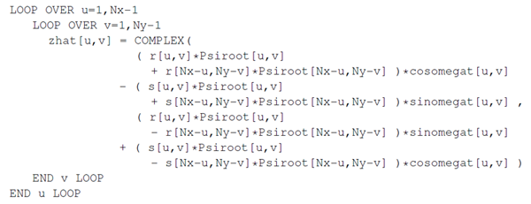
Figure 2 shows the pseudocode for looping over all values for the special case of at frequency array index . Note that for , the values are complex conjugates.
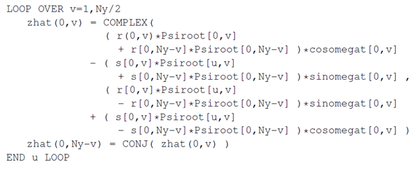
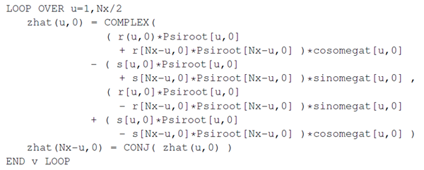
Figure 3 shows the pseudocode for looping over all values for the special cases of at frequency array index . Note that for , the values are complex conjugates.
Finally, set the value to 0, which sets the mean sea level to zero: zhat[0,0] = COMPLEX(0.0, 0.0).
Array zhat[u,v] = as just defined is Hermitian and has the frequencies in FFT order ready for input to an FFT routine.
Showing this level of detail may seem tedious, but it is absolutely critical that the array be properly computed down to the last array element. Any error will show up in the generated sea surface as either a non-zero imaginary part of the complex array (easy to detect) or an incorrect sea surface elevation (often much harder to detect).
Example: A Two-Dimensional Sea Surface
As a specific example of the above algorithm, consider the following. Let us use a coarse grid sampling of points, which makes it easier to see certain features in the associated plots. The physical region to be simulated is . The two-dimensional, one-sided variance spectrum of Elfouhaily et al. (1997) is used. Thus we have
where is the omnidirectional spectrum and is the nondimensional spreading function, as defined on page Wave Variance Spectra: Examples.
The upper left plot of Fig. 4 shows this spectrum for a wind speed of and a fully developed sea state. The contours are of evaluated at the discrete grid points; the factor seen in Eq. (2) has not yet been applied to create a discrete two-sided spectrum. The line along corresponds to the spectrum plotted in the third figure on page Wave Variance Spectra: Examples. We see in both plots that for a wind, the spectrum peaks near .
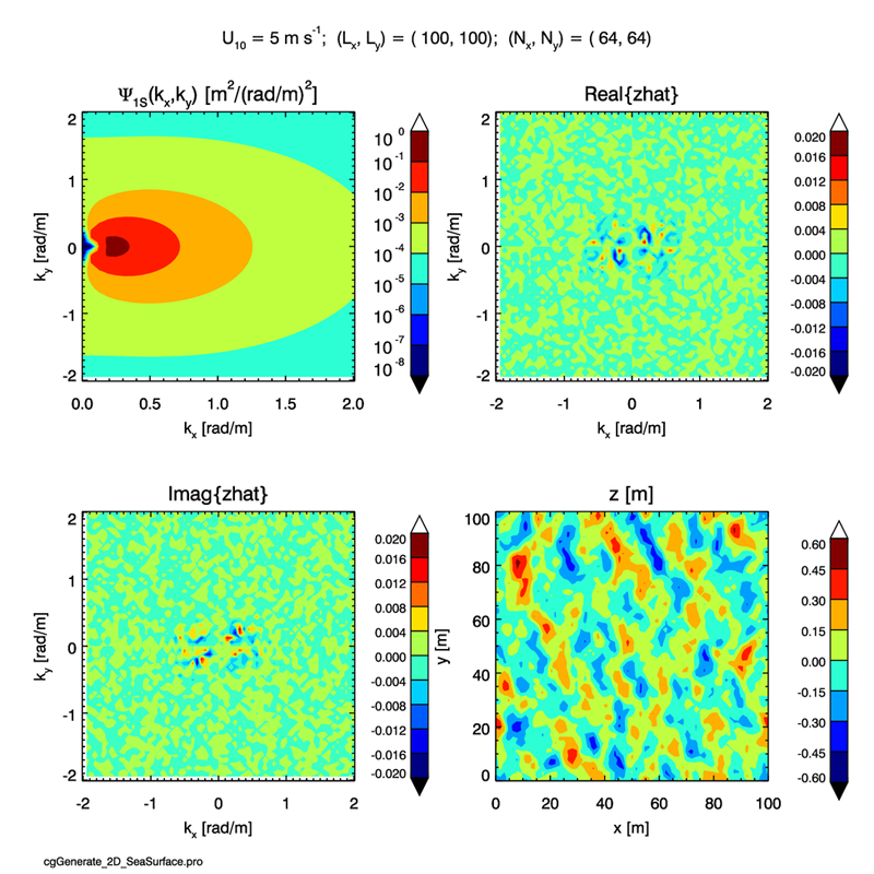
The plots of the real and imaginary parts of show that most of the variance is at low frequencies and that the amplitudes have the Hermitian symmetry illustrated in the two figures of the previous page. The lower right panel of the plot shows a contour plot of the sea surface generated from the inverse FFT of the amplitudes. The significant wave height for this surface realization is 0.60 m, in good agreement with the expected value given above for the Pierson-Moskowitz spectrum, which is similar to the Elfouhaily et al. spectrum in the gravity wave region.
 See comments posted for this page and leave your own.