Page updated:
October 13, 2021
Author: Curtis Mobley
View PDF
Mie Theory Overview
As discussed on the Physics of Scattering page, one way to change the real index of refraction and thereby cause elastic scattering is to imbed a particle of some index of refraction within a medium with a different index of refraction. If the imbedded particle is a homogeneous sphere (of any radius), the solution of Maxwell’s equations for a plane wave incident onto the sphere is now called Mie theory.
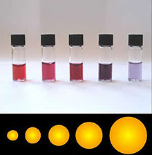
Gustav Mie (1868-1957) began his career in mathematics and mineralogy. One of the mysteries of the late 1800s was why colloidal suspensions of metallic particles displayed a rainbow of colors. Figure 2 shows an example of red to violet colors in suspensions of gold particles. The difference in colors is due to the different sizes of the gold particles, which are smaller than the wavelength of visible light. Understanding the optical effects of small concentrations of very small particles had important industrial applications because adding metallic nanoparticles to molten glass was (and still is) a common way to make glass of different colors.
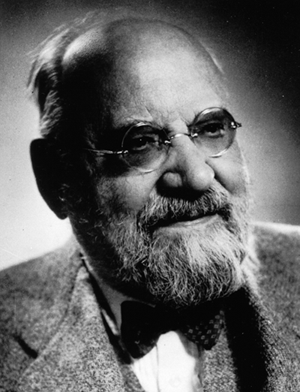
Mie approached this problem by working out the solution to scattering of light by small spheres, starting with Maxwell’s equations. His approach is all the more remarkable because, at the time, the importance of Maxwell’s equations was not yet recognized by all physicists. His classic paper, Mie (1908), is titled “Beiträge zur Optik trüber Medien, speziell kolloidaler Metallösungen,” or “Contributions to the optics of turbid media, particularly colloidal metal solutions.” Mie used his solution equations to explain how particle size and absorption properties can explain the different colors. After that success, he moved on to other problems and never published another paper on the scattering of light.
The fundamental importance of Mie’s paper went unrecognized for the next 50 years, apparently even by Mie himself. He does not even mention this paper in his autobiographical notes of 1948. This is perhaps understandable because his solution equations are so complicated that they cannot be evaluated except by modern computers. There are several short biographies of Mie, e.g.,Lilienfeld (1991) and Stout and Bonod (2020).
Statement of the Problem
This problem is formulated as follows.
- We have given a single, homogeneous sphere of radius , whose material is a dielectric with a complex index of refraction . Here is the real index of refraction, and is the complex index of refraction. The complex index is related to the absorption coefficient of the sphere material by , where is the wavelength in vacuo corresponding to the frequency of an electromagnetic wave.
- The sphere is imbedded in a non-absorbing, homogeneous, infinite medium whose index of refraction is .
- A plane electromagnetic wave of frequency is incident onto the sphere. The wavelength on the incident light in the medium is thus , which corresponds to a wavelength in vacuo of .
- We wish to find the electric field within the sphere and throughout the surrounding medium. That is, we wish to determine how the incident light is absorbed and scattered by the sphere, including the angular distribution of the scattered light and its state of polarization.
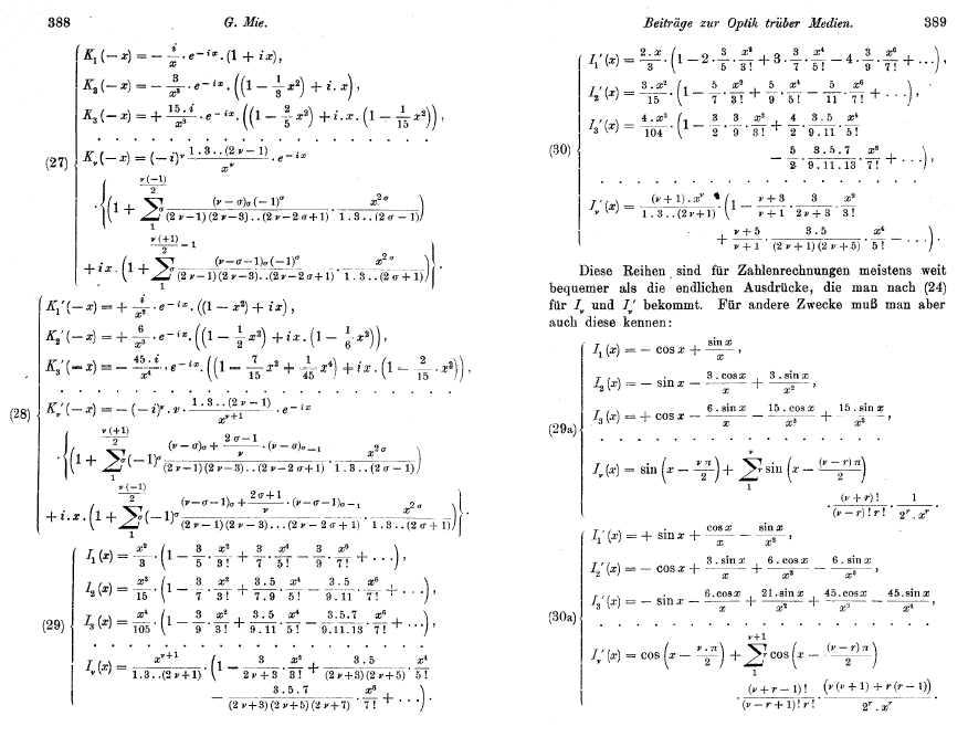
The solution of this geometrically simple problem is exceptionally difficult. Indeed, this is one of the classic problems of applied mathematics, and its solution was attempted (and partially achieved in various forms) by many of the most illustrious figures of nineteenth-century physics. For historical reasons, Mie usually gets credit for the first complete solution of the problem, and his solution of Maxwell’s equations is commonly called Mie theory. Mie’s paper, Mie (1908), is 69 pages of dense equations, and I doubt that more than a handful of people have actually read the entire paper, although it has been cited in tens of thousands of papers. Bohren and Huffman (1983) say (on page 93) that someone who works through the details of Mie’s solution will have “acquired virtue through suffering.” I second that. Mie’s paper is full of scary equations (see Fig. 4) connected by phrases like “It is easily shown that...”, “Symmetry shows that...”, and “You can convince yourself that...”
The details of Mie’s solution are given (along with much needed extra explanation and modern notation) in the texts by van de Hulst (1957) and by Bohren and Huffman (1983). The purpose of the present page is to state the problem and outline its solution, so that you will understand the inputs to and outputs from computer programs that implement Mie’s equations, and also have a qualitative idea of what is happening deep inside those programs. The following web page shows examples of Mie-computed quantities.
Geometry
Figure 3 shows the geometry of Mie theory. An incident electromagnetic plane wave (i.e., a collimated beam of light) of frequency (cycles per second) is incident onto a homogeneous spherical particle at the origin of a coordinate system. The coordinate system is chosen so that the wave is propagating in the direction, and the origin of the coordinate system is chosen so that the wave is a cosine at time 0. The incident electric field in the medium of real index of refraction then can be written as
where is the wavenumber (cycles per meter) in the medium, and is the angular frequency (radians per second). is the amplitude of the incident electric field vector, and the direction of propagation is . Life will be mathematically easier later on if we write the incident wave as a complex variable,
and keep in mind that we’re interested in only the real part of the complex variable . We’re dealing with Maxwell’s equations, which involve both electric and magnetic fields. However, if you know one, then you can get the other, so it suffices to discuss just the electric field.
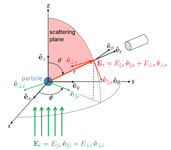
The incident wave will interact with the particle at the origin of the coordinate system and generate a scattered wave traveling in direction , which is at polar and azimuthal angles as seen in Fig. 3. The incident direction and the scattered direction define the scattering plane, part of which is shaded in pink in the figure.
Light is a transverse electromagnetic wave, which means that the electric and magnetic fields are perpendicular to the direction of travel. The incident wave is also arbitrarily polarized. An arbitrary state of polarization of can be written as a combination of two components, which are orthogonal to the direction of propagation. We choose these two directions to be parallel and perpendicular to the scattering plane. Thus we can write the incident electric field as
| (1) |
where the parallel () and perpendicular () directions are shown by the thin green arrows in Fig. 3. Note that . At large distances from the particle (the so-called “far field”), the scattered field becomes transverse and can also be written as a combination of components in directions parallel and perpendicular to the scattering plane: . The directions and are parallel and perpendicular to the scattering plane at the point where the scattered light is being measured by an instrument looking towards the particle at the origin. As seen in Fig. 3, but . In particular,
where give the directions of increasing in the spherical coordinate system.
The Solution
For an arbitrary (i.e., non-spherical and/or inhomogeneous) particle at the origin, the scattered wave can be written as
| (2) |
The four are the elements of the amplitude scattering matrix. These functions transform the amplitudes of the incident electric field into the amplitudes of the scattered field. For an arbitrary particle, all four elements of the amplitude scattering matrix are non-zero and depend on both the polar and azimuthal scattering angles. These functions of course depend on the particle size, shape, and composition, as well as on the wavelength of the incident light, and it is that dependence that we wish to determine.
This present discussion accepts the form of Eq. (2) as given to us by the physicists, but it is worth a comment. When working with 3D waves, it is common to seek a solution that separates the radial and angular variables. Here the depend only on . The irradiance of an electromagnetic wave is proportional to square of the amplitude of the electromagnetic field. Squaring Eq. (2) gives a factor of
We are considering scattering by a single particle, so the farther away we are from the particle, the less the irradiance detected by a sensor looking at the particle will be by a factor of . This result is known as the “ law for irradiance.” We see here how the form of (2) for the scattered field has the law for irradiance built into the radial dependence of the electric field amplitudes. In particular, we are interested in the “far field” of the scattered light, which means that . Note also that since is non-dimensional, so must be the matrix elements.
For a homogeneous spherical particle, and the amplitude scattering matrix reduces to
| (3) |
Now comes the hard part: how to compute and given the particle radius , the complex index of refraction of the spherical particle, , and the real index of refraction of the medium, .
[Comment on notation. It is common in Mie theory papers to use as the radius of the spherical particle. However, in applications of Mie theory to optical oceanography, that leads to confusion with the absorption coefficient. Mie used , and that’s good enough for me (pun intended). There is also confusion between the common use of as wavenumber and as the complex part of the index of refraction; Bohren and Huffman use a Roman for wavenumber and an italic for the imaginary part of the index of refraction. I avoid that subtlety by using for wavenumber and for the imaginary part of the index of refraction of the sphere, but then I’m using a subscript for both “sphere” and “scattered,” although context should keep things clear. Bohren and Huffman use for the phase shift paramenter . Choosing good notation is a never-ending problem.]
The incident and scattered electric fields must satisfy both Maxwell’s equations and boundary conditions for the behavior of the electric field at the surface of the sphere and at infinity. It is these boundary conditions that determine exactly which of all possible electric fields that satisfy Maxwell’s equations is the one particular field that describes scattering by a particular sphere.
Figure 4 shows a couple of the pages of Mie’s 1908 paper. This figure should be sufficient to convince you that we should skip the mathematical details and jump straight to the answer.
Mie’s solution is in the form of infinite series of very complicated mathematical functions. The terms in these series depend on a size parameter ,
| (4) |
and the refractive index of the sphere relative to that of the surrounding medium,
| (5) |
The size parameter is a measure of the sphere’s size relative to the wavelength of the incident light in the surrounding medium. This parameter shows why oceanographers tend to use wavelength rather than frequency as the measure of light’s oscillations: it is particle size relative to wavelength that is important for scattering (whether or not the particle is spherical). Note that the real part of the relative refractive index can be less than 1, for example if the spherical particle is an air bubble () in water ().
Mie’s solution (in modern notation) is
where
The and are often called the “Mie coefficients.” These functions describe multipole expansions of the electric () and magnetic () fields of the scattered wave: is the dipole term, is the quadrapole term, and so on. The and are Riccati-Bessel functions; the prime denotes derivatives of these functions with respect to the argument of the function (either or ). Riccati-Bessel functions are obtained from something called spherical Bessel and spherical Hankel functions, which in turn are obtained from something called Bessel functions of the first and second kind, which are themselves.... You get the idea. You eventually get down to something normal people can understand, likes sines and cosines. The and are angle-dependent functions obtained by recursion relations:
starting with and .
Thus the amplitude functions and depend on the particle size and index of refraction via the and in the and , and on scattering angle via the factors in and . For the geometry of Fig. 3, the polar angle is the scattering angle ( is my preferred symbol for scattering angle), and the results are independent of the azimuthal scattering angle because of the symmetry of the sphere. It should be noted that if , i.e., if the sphere has the same index of refraction as the surrounding medium, then and for all . That is to say, there is no scattering. This observation highlights that scattering is caused by differences in index of refraction.
Mie Theory is exact and valid for all sizes of spheres, indices of refraction, and wavelengths.
However, it is not possible to compute the sums of the infinite series (6) analytically. The sums must be approximated numerically by adding only a finite number of terms in the series. If the size parameter is less than roughly 10, e.g. typically when , only the first few terms are needed to get an accurate approximation for and . However, for large size parameters, e.g. when , many terms must be computed and convergence of the series is very slow. A well established rule seems to be that the number of terms that must be computed is the integer closest to
Suppose we want to compute scattering by a spherical phytoplankton of radius , real index of refraction , in water with , at a wavelength of . The size parameter is then and . That is no problem for a computer. But suppose we want to compute the scattering for a rain drop of size , , in air with , and for . Then and . That can take a while.
[The BHMIE code used to generate the examples on the next page is restricted to for reasons of computational accuracy. However, specialized codes have been designed for use with size parameters larger than , but you are then getting into the world of quadruple-precision arithmetic and supercomputers.) In Mie’s original paper, he had to do the calculations by hand. He was able to compute only the first three terms of the infinite series, which limited his applications to particles less that 200 nm in size for visible wavelengths ( of order 1). However, that was sufficient to explain the optical effects of scattering by the colloidal particles that prompted his study.]
It must be remembered that and are complex variables that transform incident complex electric fields into scattered complex electric fields. In oceanography, we are interested in scattered energy, which can be detected and turned into radiances. We are also interested in the shape of scattering phase function as a function of scattering angle, and in other quantities like absorption and scattering coefficients. The energy in an electric field is proportional to its amplitude squared so, not surprisingly, the quantities of real interest are obtained from various functions of the absolute values squared of and . The are real functions that are proportional to the scattered power (i.e., to scattered irradiance).
Suppose that the incident light is polarized parallel to the scattering plane, i.e. in Eq. (1). Then Eq. 2 shows that for an arbitrary particle, this incident light can be scattered into light that has components that are both parallel and perpendicular to the scattering plane. But for a spherical particle, Eq. 3 shows that incident light polarized parallel (perpendicular) to the scattering plane is scattered into light that remains polarized parallel (perpendicular) to the scattering plane.
Thus the angular pattern (ignoring normalization factors) of the incident parallel-polarized light that is scattered parallel to the scattering plane is given by
where denotes complex conjugation. Likewise the perpendicular-incident to perpendicular-scattered pattern is given by . It is therefore common to plot and as functions of the scattering angle to see how these two polarization states are scattered.
and can be thought of as unnormalized scattering phase functions for particular states of polarization. The oceanographer’s scattering phase function for unpolarized light is, to within a normalization factor, given by
| (9) |
A word of warning here: Mie codes return and for the set of scattering angles requested by the user (e.g., from 0 to 180 deg by 0.1 deg). You can then use Eq. 9 to compute the phase function, but you can be guaranteed that it will be unnormalized. For example, if you study Bohren and Huffman (and you should), you will see many places where they say something like “where we have omitted the factor ” (page 113). You need to integrate the obtained from 9 to determine the needed normalization factor. A phase function used in a radiative transfer code such as HydroLight must satisfy the normalization .
Additional output of Mie codes is usually given as various absorption and scattering efficiencies. The absorption efficiency , for example, gives the fraction of radiant energy incident on the sphere that is absorbed by the sphere. The term “energy incident on the sphere,” means the energy of the incident plane wave passing through an area equal to the cross-sectional (projected, or “shadow”) area of the sphere, . Likewise, the total scattering efficiency gives the fraction of incident energy that is scattered into all directions. Other efficiencies can be defined: for total attenuation, for backscattering, and so on.
Mie solutions may also be presented in terms of absorption and scattering cross sections. The physical interpretation of these cross sections is simple. The absorption cross section , for example, is the cross sectional area of the incident plane wave that has energy equal to the energy absorbed by the sphere. The absorption and scattering cross sections are therefore related to the corresponding efficiencies by the geometrical cross section of the sphere. Thus
Likewise, , and so on for , etc.
For the record, these cross sections are obtained within the Mie code from the and functions of Eq.(7):
where denotes the real part of the argument; is equivalent to ).
The cross sections obtained from Mie theory are for a single particle and have units of per particle, for the given particle properties. In oceanography, we are usually interested in a water body containing a huge number of particles per cubic meter. If there are particles per cubic meter corresponding to particle radius (for given other conditions of indices of refraction and wavelength, which determine the size parameter and relative index of refraction ), then the oceanographers’ scattering coefficient corresponding to a collection of identical particles is
Now, of course, the ocean does not contain just one size and type of particle. The range of particle sizes is described by the particle number size distribution , where is a function such that the number of particles with radii between and is . The units of are particles per cubic meter per size interval, which is usually written as because particle sizes are usually measured in micrometers. Particle size distributions are often modeled as a power law of the form , where sets the scale and is in the range of 4 or 5. So the total scattering coefficient due to all particles of a given type is then
In practice, the integration over all will be approximated as a summation from some minimum size to some maximum size for which the term makes a significant contribution to the summation.
There will also be different types of particles for a given size , which gives different and parameters in the Mie equations, hence different cross sections for the different particle types: , where labels the type of particle (cyanobacteria, quartz sand, etc.). Each particle type can have its own size distribution, . Then the total scattering coefficient for all sizes of all particle types is
| (10) |
Thus there must be many evaluations of the Mie equations to obtain the cross sections for a realistic range of particle types and size bins. Keep in mind that if Mie theory is used to obtain the cross sections, then it is being assumed that the particles are homogeneous spheres, which is almost never the case in the ocean. However, Eq. (10) shows how Mie calculations can be used to compute the quantities used in optical oceanography if the particles can be approximated as homogeneous spheres.
As a final comment on Mie theory, Mie codes often output something called the “radar cross section.” This is the hypothetical area required to intercept incident power onto the particle such that if the total intercepted power were re-radiated isotropically with a scattering amplitude equal to the amplitude for exact backscattering (at 180 deg), the power actually observed at the receiver is produced. Do not confuse this quantity with the backscatter cross section , which corresponds to scattering over the backward hemisphere of the phase function without any assumption of isotropic scattering pinned to the phase function value at 180 deg. Most Mie codes unfortunately call the radar cross section the backscatter cross section in their output files, which leads to much confusion. See Bohren and Huffman (1983) Section 4.6 for further discussion.
The next page shows example output from a Mie computer code.
 See comments posted for this page and leave your own.