Page updated:
November 13, 2021
Author: Curtis Mobley
View PDF
Mie Theory Approximations
Curtis Mobley and Emmanuel Boss contributed to this page.
As discussed on the previous two pages, Mie theory is exact for homogeneous spheres of any size, but it can be computationally expensive, especially for spheres that are large relative to the wavelength of the light incident on them. There are, however, analytical approximations to the exact theory that can be useful in limited situations. Loosely speaking, these might be called approximations for “really small particles,” “weakly scattering particles,” and “really large particles.” This page presents these three approximations and illustrates the limits of each.
Small Particles, : Rayleigh’s Approximation
John William Strutt had the good fortune to be born a wealthy British aristocrat at a time when that still meant something. Unlike some of his peers, he did not spend his life in the idle dissipation of an inherited fortune. Indeed, he became one of Britain’s greatest scientists. He worked in many areas including optics, acoustics, and fluid mechanics, publishing 446 papers. He received many honors, including the Nobel Prize in Physics in 1904 for “for his investigations of the densities of the most important gases and for his discovery of argon in connection with these studies.” Upon the death of his father in 1873, he inherited the title of Baron Rayleigh, and was henceforth known as Lord Rayleigh. Masters (2009) gives a short biography of his scientific life.
In a series of three papers published in 1871, he developed equations to describe scattering by non-absorbing particles that are small compared to the wavelength of the incident light. The first of these papers, Strutt (1871), titled “On the Light from the Sky, its Polarization and Colour,” begins “It is now, I believe, generally admitted that the light which we receive from the clear sky is due in one way or another to small suspended particles which divert the light from its regular course.” He first used dimensional analysis to conclude that the scattering must be proportional to the inverse fourth power of the wavelength. He then went on to work out the mathematics in full.
Rayleigh found, under the assumption that the particle is much smaller than the wavelength of the incident light, that the single-particle volume scattering function for unpolarized light (to use modern terminology and notation) is
| (1) |
where is the particle radius, is the wavelength, is the real index of refraction of the particle relative to that of the surrounding medium, and is the scattering angle. This result can be written as the product of a single-particle scattering cross section and a scattering phase function , , where
This phase function satisfies the normalization condition . Note that has units of . After multiplication by particles per cubic meter, the result is a scattering coefficient with the customary units of inverse meters. describes the angular scattering per steradian, so the bulk VSF then has units of . Dividing by the particle cross section and rewriting in terms of the Mie theory size parameter (for a medium index of refraction of 1) gives the scattering efficiency
| (4) |
Rayleigh used the dependence of his equations to explain the blue sky as wavelength-dependent scattering by the “small suspended particles” of his first papers. However, in Rayleigh (1899) he returned to “...the interesting question whether the light from the sky can be explained by diffraction from the molecules of air themselves, or whether it is necessary to appeal to suspended particles composed of foreign matter, solid or liquid.” and concluded that “...even in the absence of foreign particles we should still have a blue sky.”
Rayleigh’s approximation obtained from Mie theory
Rayleigh’s result (1) can be obtained from and extended by Mie theory, which came 36 years later. Recall from the equations of the Mie Theory Overview page that Mie’s solution for scattering by a sphere is in the form of infinite series, the terms of which depend on powers of the size parameter . Expanding the series solution and keeping terms through eventually leads to the efficiency factors (See Bohren and Huffman (1983) §5.1 for the math)
| (5) |
and
| (6) |
where now the index of refraction can be complex, i.e. the sphere can be absorbing. and indicate the real and imaginary parts of the quantities in braces, and indicates the absolute value squared of the complex quantity. If the particle is non-absorbing, is real. The first term in Eq. (5) is then zero, and the second term is then the same as Eq. (6) and Rayleigh’s seen in Eq. (4). The Rayleigh scattering coefficient (in the form of either , , or ) thus falls out of the first terms of the Mie solution. If is small enough that terms of order and higher can be ignored, then the absorption efficiency reduces to just
| (7) |
Remembering that , then if the factor is almost independent of wavelength over some wavelength interval, then and over that interval.
Applicability of Rayleigh’s approximation
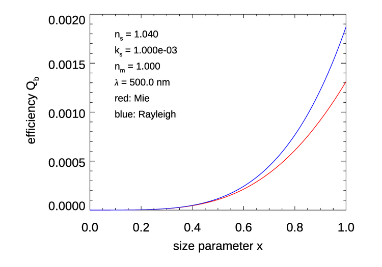
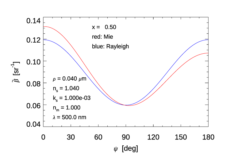
Rayleigh’s scattering result (4) was derived for very small, non-absorbing particles. The question remains as to how small is small enough for the Rayleigh formulas to be accurate within some error compared to the exact Mie theory. In particular, can Rayleigh’s equations be used to compute scattering by phytoplankton or other oceanic particles? At visible wavelengths, phytoplankton typically have real indices of refraction in the range of 1.02 to 1.1, relative to water (e.g., Ackleson and Spinrad (1988)). The complex index of refraction is in the region of 0.001 at 500 nm up to 0.005 in an absorption band (e.g., Table 1 of Bricaud et al. (1983)). Figure 1 compares the Mie and Rayleigh scattering efficiencies for a typical phytoplankton index of refraction and a wavelength of 500 nm. (The Mie calculations for this figure and the following ones were done with the IDL version of the Bohren and Huffman Mie code (BHMIE) downloaded from the SCATTERLIB website.) Suppose we accept a 10% error in as an acceptable trade-off for the ease of computation. For a size parameter of , the Rayleigh is about 9% too large. Figure 2 shows the corresponding difference in phase functions for . Again, the maximum difference is about 10% (at and 180 deg). So we could use the Rayleigh formulas for size parameters up to 0.5 for phytoplankton. The problem for oceanography is that a size parameter of for gives a particle radius of , which is an order of magnitude smaller than bacteria or the smallest phytoplankton. Thus the Rayleigh scattering formulas are not useful for computing the scattering coefficients or phase functions for phytoplankton or other oceanographic particles, which are usually of size or larger.
Comment: Rayleigh was not the first to recognize that scattering by very small particles was a primary contributor to the blue of the sky; he was the first to work out the physics and math. His work captured much, but not all, of the physics of Earth’s sky color. We now understand that the “small suspended particles” assumed by Rayleigh are mainly the nitrogen and oxygen molecules that comprise most of the atmosphere. To really understand sky color, in addition to the scattering law, one must also take into account the wavelength dependences of the solar spectrum and the response of the human eye. The excellent text by Bohren and Clothiaux (2006) devotes much a chapter to the blue-sky problem, including absorption by ozone at green to red wavelengths. See also Bohren and Fraser (1985) for a non-mathematical summary. That Rayleigh did not totally account for every last contribution to the color of the sky in no way detracts from the brilliance of his work at age 29, in an era when light was still supposed to propagate through a “luminiferous aether” and the very existence of atoms and molecules was disputed by many eminent scientists. (The debate about whether atoms and molecules actually exist, or whether they are just convenient mathematical artifices, was quite acrimonious. The great Ludwig Boltzmann became so depressed trying to convince people that his statistical mechanics proved that molecules are real entities that he committed suicide in 1906.)
Weakly Scattering or “Soft” Particles: The Rayleigh-Gans Approximation
A second approximation to Mie theory is available for particles whose complex index of refraction relative to the surrounding medium, , and size parameter satisfy two conditions:
These are two independent requirements. says that the particle scatters only weakly; there would be no scattering if the real part of the index of refraction were exactly 1. says that the particle is small enough that there is only a small change in the phase and amplitude of the incident electromagnetic wave as it passes through the particle. That is, the electric field inside the particle is almost the same as that of the incident wave. is usually called the phase shift parameter. Particles that satisfy Eqs. (8) and (9) are usually called optically “soft” particles. Recall that Rayleigh’s equations require that the particle size parameter be small. The Rayleigh-Gans simplification allows to be large so long as the index of refraction is small enough to satisfy .
To develop the solution, the volume of the particle is divided into small volume elements. The particle does not need to be spherical. Each volume element receives essentially the same incident electromagnetic wave (condition (9)), which it then scatters according to the Rayleigh approximations for . However, there will be phase differences for the scattered waves from different volume elements, which lead to interference effects. These are accounted for via an integration of the phase differences over the volume of the particle. The result of that integration is a non-dimensional form factor , which depends on both the polar () and azimuthal () scattering angles if the particle is non-spherical. The form factor contains all of the information about the shape of the particle.
The scattering-matrix elements have the same general form as those obtained from Mie theory (see Eq. (3) of the Mie Theory Overview page), except for extra factors of ; see Bohren and Huffman (1983) §6.1 for the details. These matrix elements eventually lead to a phase function for scattering of unpolarized light of the form
| (10) |
where is the volume of the particle, and is the proportionality constant that normalizes the phase function; this is easily computed by numerical integration after the rest of the calculations are performed. This equation holds for any shape of particle.
As noted, must be computed by an integration over the volume of the particle. For a homogeneous spherical particle, depends only on the polar scattering angle, and the integration can be done analytically with the result
| (11) |
Although the phase function of Eq. (10) contains a factor like that of the Rayleigh phase function of Eq. (3), the form factor makes the Rayleigh-Gans phase function much more peaked at small scattering angles.
Let the index of refraction of the particle relative to the surrounding medium be written as and define a parameter by
| (12) |
Note that ranges from 0 (for non-absorbing particles) to (for absorbing particles with approaching 1). Then the Rayleigh-Gans extinction and absorption efficiency factors for spherical particles are functions of and the phase shift parameter :
For nonspherical particles, the Rayleigh-Gans scattering efficiency factor depends on the polarization state of the incident light. For a spherical particle, the scattering efficiency can be obtained from the preceding two equations. For non-absorbing particles, , and Eq. (13) reduces to just
| (15) |
Applicability of the Rayleigh-Gans approximation
To give an idea of its applicability in oceanography, Fig. 3 compares the Rayleigh-Gans efficiency factors with those of the exact Mie numerical calculations for typical phytoplankton IOPs. The Rayleigh scattering or extinction efficiency of Eq. (4) is also shown, as is the equivalent Rayleigh absorption efficiency of Eq. (7), obtained from the lowest-order term of the Mie series expansion. The figure displays the results as a function of the phase shift parameter . Not surprisingly, the Rayleigh scattering efficiency blows up for , corresponding to . However, the Rayleigh-Gans equations do very well for much larger values. (For these IOPs, corresponds to a size parameter of .) This is quite unexpected and remarkable given that Rayleigh-Gans theory was developed on the assumption than . Indeed, van de Hulst (1981) on page 176 comments on Eq. (15) that “This is one of the most useful formulae in the whole domain of the Mie theory, because it describes the salient features of the extinction curve not only for close to 1 but even for values of as large as two.” The same holds for Eqs. (13) and (14).
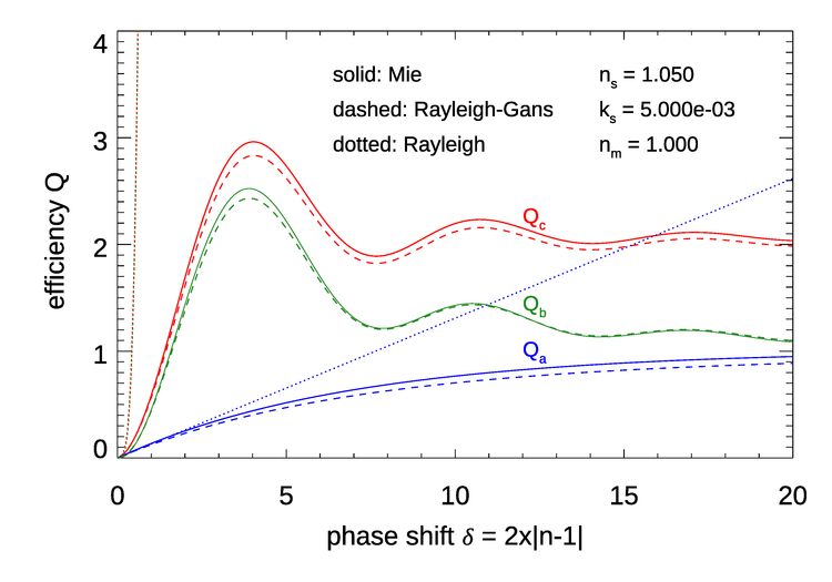
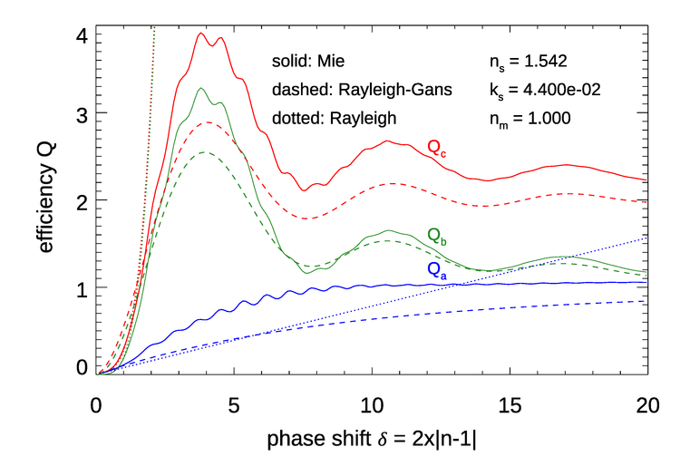
Figure 4 shows the efficiencies for the IOPs typical of soot; recall Fig. 6 of the Mie Theory Examples page. Even for this high-index-of-refraction, highly absorbing particle, Rayleigh-Gans does amazingly well. (For these IOPs, corresponds to a size parameter of .)
Because of their wide range of validity, the Rayleigh-Gans efficiency formulas have been used to gain insight into phytoplankton optical properties. Examples are Bricaud et al. (1983) and Gordon (2007).
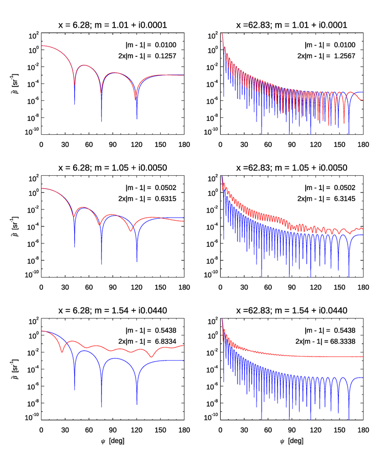
Now consider how well Rayleigh-Gans phase functions computed by Eqs. (10) and (11) compare with the exact Mie phase functions. Picoplankton have diameters on the order of , or ; nanoplankton have diameters of order . For a wavelength of , these give size parameters of and 62.8, respectively. Figure 5 compares exact Mie and Rayleigh-Gans phase functions for these size parameters and indices of refraction that are very near 1, ; typical of phytoplankton, ; and typical of soot, . For the very low index (top two figures), the envelopes of the maximum values of the Rayleigh-Gans phase function are close to those of the Mie phase functions. For the large particle (upper right plot), the peaks are somewhat out of phase for large scattering angles, but this is probably acceptable for most applications because a disperse range of sizes would cause the individual interference features to average out, leaving only the upper bound of the curves (recall Fig. 5 of the Mie Theory Examples page). By the same argument, the Rayleigh-Gans phase function for the small size, typical index particle (middle left figure) would be acceptable for many applications. However, the large-phytoplankton phase functions (middle right figure) differ by an order of magnitude over almost the entire range of scattering angles. Averaging over a range of sizes will not bring those curves together. Similarly, for the high-index soot particles (bottom row), Mie and Rayleigh-Gans differ by one or two orders of magnitude for most scattering angles. Thus it seems that, although Rayleigh-Gans efficiency factors perform well beyond the range of their derivation, the Rayleigh-Gans phase functions cannot be pushed as far.
Large Particles, : Geometric Optics
At the other end of the size spectrum are particles that are much larger than the wavelength of the light incident onto them. This is the realm of geometrical optics and ray tracing. The needed tools are simply Snell’s law, Fresnel’s law, and a computer. Geometric ray tracing can compute the optical properties, phase functions in particular, for any shape of particle, but at the expense of missing any effects due to diffraction or interference. For visible wavelengths, diffraction can be significant for particles in the size range of most phytoplankon, or . For diffraction to appear insignificant compared to reflection and refraction, particle sizes need to be of order 0.05 mm or larger, which gives a size parameter of . Thus ray tracing is seldom used of computing the phase functions of oceanic particles. However, ray tracing is commonly used to compute the reflectance and transmission properties of wind-blown sea surfaces (e.g., Mobley (2015)) or of underwater objects or surfaces (e.g., Mobley (2018)).
In geometric optics ray tracing, a ray that misses a particle by even the smallest distance continues onward unperturbed. Consider a particle that is so highly absorbing that it absorbs all of the light that hits it. Then no light will be scattered. The absorption and scattering efficiencies are then and , so that the extinction efficiency . Conversely, if the particle is non-absorbing, all light that hits it will be scattered. Then , , and . This is the origin of the “extinction paradox,” which was discussed on the Mie Theory Examples page. There we saw that Mie theory leads an asymptotic large-particle value of , not 1. The difference is that Mie theory fully accounts for diffraction and interference effects, and geometric optics does not.
Incidentally, if you want to convert a geometric optics efficiency into a cross section , there is a wonderful result, Cauchy’s Average Projected Area Theorem, which shows that for a convex polyhedron, the average projected area over all orientations, i.e. the average cross section, is one-fourth the surface area of the polyhedron. (This result is obvious only for a sphere, whose surface area is and whose cross section is .) If is the average area of the particle as seen from all orientations, the the cross section is given by , regardless of the particle shape (as long as it is convex, i.e., without any “indentations” in its surface).
A geometric optics ray tracing example
The use of ray tracing to explain rainbows goes back to Descartes in the early 1600s. Another area of geophysical optics where ray tracing has proved very useful is the computation of phase functions for atmospheric ice crystals in cirrus clouds. These clouds are important for modeling the Earth’s radiation balance. Ice has a hexagonal crystal structure, so cloud ice crystals commonly form as hexagonal plates or solid or hollow columns, although more complex shapes (e.g., snowflakes and columns with pyramidal caps or indentations) can form, depending on the temperature and humidity during formation.
Figure 6 illustrates possible ray paths through a solid hexagonal column of ice, which is very common in cirrus clouds. Such columns are on the order of 0.05 to 0.5 mm in size. When ray tracing through such columns, millions of rays are traced for randomly oriented columns. The reflected and refracted rays for different directions are then used to build up, ray by ray, the shape of the scattering phase function. Certain directions, such as those shown by the red and green arrows in Fig. 6, tend to generate caustics, or “collections” of rays near particular directions (just as happens for spherical water drops in the formation of rainbows).
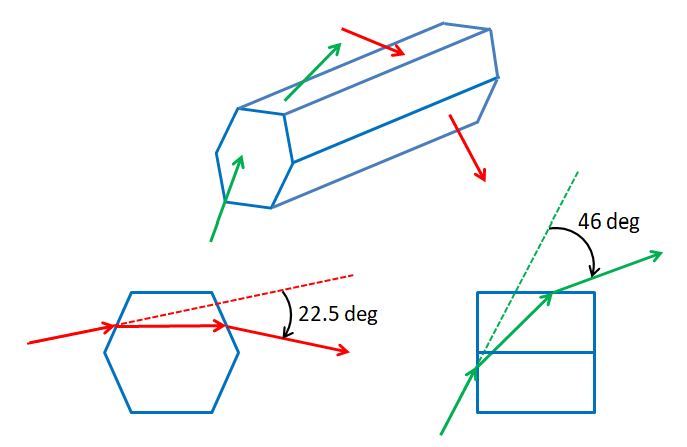
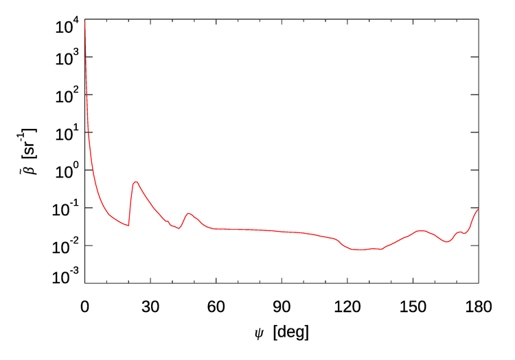
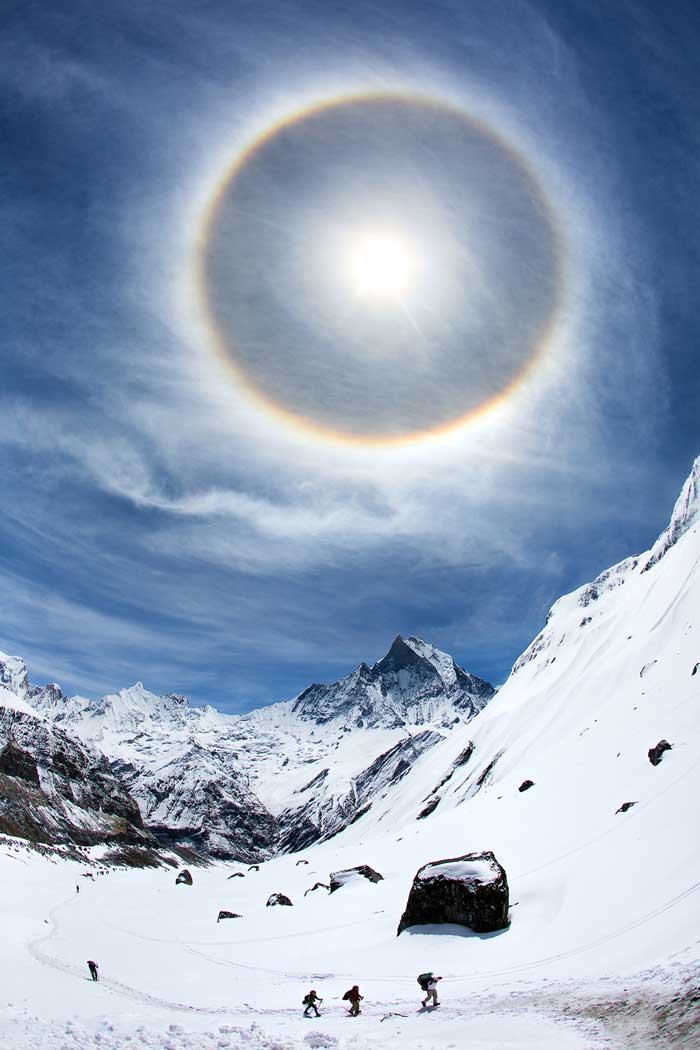
Figure 7 shows the scattering phase function for cirrus clouds containing hexagonal columns like those of Fig. 6. The prominent peaks near 22 and 46 degrees give a halo or “ring around the Sun” (or Moon) at those angles. The 22 deg halo is common. The 46 deg halo, resulting from rays passing through the flat ends of hexagonal column, is seen less often. The peak near 160 deg results from two internal reflections in the crystal. Figure 8 shows a spectacular 22 deg halo. Note how well the phase function of Fig. 7 matches the halo: There is a very sharp transition from darker to brighter on the inner side of the halo, where the phase function rises very rapidly between and 22 deg. Then there is a slower decrease in brightness on the outer side of the halo, corresponding to the slower decay of the phase function between 23 and 44 degrees. There is no 46 deg halo in this image. That will be the case if the hexagonal crystals do not have the flat ends needed to create the 46 deg peak in the phase function, as illustrated by the green rays in Fig. 6. The color in the halo results from the small difference in the ice index of refraction as a function of wavelength.
A myriad of other halos can be generated by ice crystals of other shapes. Some of these crystal shapes rarely form and the resulting halos are almost “once-in-a-lifetime” events. An excellent book showing photographs of many types of halos, rainbows, glories, and other atmospheric phenomena, along with explanations of their causes, is Greenler (2020). There are free ray tracing codes for halo simulation now available, e.g., HaloSim 3 and HaloPoint 2.
Closing Thoughts
Rayleigh developed his scattering theory in the late 1800s, and it worked quite well to solve the problem of interest to him. Rayleigh-Gans theory arose in the late 1800’s and early 1900’s. (Gans worked out the theory for homogeneous spheres in 1925.) In those pre-computer days, use of the exact Mie theory was not possible, so analytical approximations were the only option for computation of scattering properties of particles. As we have seen, Rayleigh scattering theory is not applicable to scattering by oceanic particles like phytoplankton or mineral, which are too large. Rayleigh-Gans theory does have some usefulness, but it too has its limits. Geometric optics can be useful for atmospheric particles like large ice crystals, but oceanic particles tend to be too small for geometric optics. Thus the approximations surveyed on this page are of interest, but they do not find frequent application in oceanic optics. There are additional analytical approximations for spherical particles, but these have found little if any application in optical oceanography. Those approximations are surveyed in Kokhanovsky and Zege (1997). If you have spherical particles, it is usually feasible with modern computers to do numerical Mie calculations without the need for approximations. For non-spherical particles, there are other numerical methods that can be used (e.g., T-matrix theory or the discrete dipole approximation).
It should be noted that this page refers to “Rayleigh’s approximation” and “the Rayleigh-Gans approximation,” rather that to “Rayleigh scattering,” or “Rayleigh-Gans scattering,” as is commonly seen. This is to emphasize that “Rayleigh scattering,” “Rayleigh-Gans scattering, and Geometric optics are not physically different types of scattering. They are approximate mathematical models for computing scattering quantities such as cross-sections and phase functions in particular size and index-of-refraction domains. As explained on the Physics of Scattering page, all scattering is caused by a change in the real index of refraction and in that sense all scattering is fundamentally the same.
 See comments posted for this page and leave your own.