Page updated:
April 5, 2021
Author: Curtis Mobley
View PDF
K functions
We now further examine the diffuse attenuation functions, which are commonly called “K functions.” Recall, for example, the definition of the diffuse attenuation function for downwelling plane irradiance:
Solving this for the irradiance gives
This equation is exact. If were independent of depth — which it never is, as will be seen below — the last equation would reduce to
This equation is always an approximation. Corresponding equations can be written for all other radiometric variables and their corresponding K functions..
Under typical oceanic conditions, for which the incident lighting is provided by the Sun and sky, and in homogeneous water, when far enough below the surface (and far enough above the bottom, in optically shallow water) to be free of boundary effects, the K functions do become almost independent of depth, in which case the various radiances and irradiances all decrease approximately exponentially with depth. The assumption of an exponential decrease of the light field with depth is often good enough for a back-of-the-envelope estimation, but it must always be remembered that reality is more complicated.
Dependence of K Functions on IOPs and Environmental Conditions
As explained in the previous page, in order to be useful for relating light measurements to water properties, the K functions should depend strongly on water IOPs but only weakly on external environmental conditions like Sun location, sky condition, or surface waves. To illustrate these dependencies, various K functions were numerically computed using the HydroLight radiative transfer numerical model. In most situations it is preferable to work with real data. However, use of this model gives us the ability to simulate different environmental conditions at will and to control things that cannot be controlled in nature, such as turning chlorophyll fluorescence on or off to see its effect. This can be very useful for understanding the interdependence of various quantities.
HydroLight simulations were first performed at one wavelength for homogeneous idealized water bodies dominated by either scattering or absorption. For the “highly scattering” water, the absorption coefficient was set to , and the scattering coefficient was , so that the albedo of single scattering was . These values correspond roughly to what might be found at blue or green wavelengths in Case 1 water with a chlorophyll concentration of . An “average-particle” scattering phase function was used, the Sun was placed in a clear sky, and the water was infinitely deep. Note that since , the nondimensional optical depth is numerically equal to the geometric depth in meters.
Figure 1 shows various K functions as a function of depth for the highly scattering water when the Sun was placed at a zenith angle of 40 degrees and the surface was level (wind speed of ). As is conventional in radiative transfer theory, the curves are for radiance propagating in the direction. HydroLight measures depth positive downward from the mean sea surface, and polar angle is measured from the or nadir direction. Thus refers to light heading straight down into the water (corresponding to ), refers to light heading straight up (corresponding to , and refers to light traveling horizontally through the water. Azimuthal angle refers to light heading towards the Sun, which was placed at ; thus refers to light heading away from the Sun. In this simulation, corresponds to looking into the Sun’s refracted beam underwater, which is light heading downward and away from the Sun.
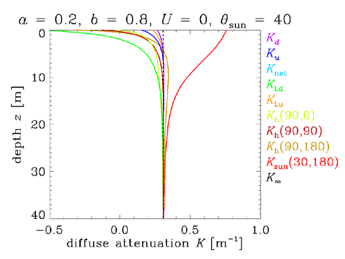
There are several important features to note in Fig. 1:
- The various K functions can differ greatly near the sea surface. This due to boundary effects on the solution of the radiative transfer equation. The surface boundary affects radiances in different directions in different ways depending on the relative location of the sun. The large near-surface values of indicate that the Sun’s direct beam is decreasing rapidly with depth due to absorption and scattering out of the beam. On the other hand, , which is looking straight downward at radiance propagating upward, is almost constant with depth.
- K functions can be positive or negative near boundaries. A negative K means that the radiometric variable is increasing with depth. , which is looking in the zenith direction at radiance propagating downward, is negative in the first few meters below the surface. At depth 0 just below the sea surface, the downwelling radiance comes mostly from the zenith sky radiance transmitted through the level surface. Going deeper into the water, increases with depth as scattering from the Sun’s strong direct beam contributes more path radiance to than is lost by absorption and scattering out of the downward beam. Eventually the Sun’s direct beam becomes weak enough that the path radiance contribution to is less than the attenuation due to absorption and scattering out of the beam, and becomes positive. The same effect is seen less dramatically in , which corresponds to looking horizontally toward the Sun.
- K functions are not constant with depth even in homogeneous water. Again, this is a manifestation of the surface boundary effects. If the water IOPs depend on depth, then the K functions also vary with depth, even far from a boundary. Thus radiometric variables never decrease exactly exponentially with depth, although this is often a good approximation for homogeneous water.
- Far from boundaries (i.e., very deep in the ocean and very far from the bottom), all K functions approach a common value, the “asymptotic K value” , that depends only on the IOPs. Its value for the IOPs of this simulation was . Thus at depths great enough for boundary effects to be negligible, all K functions are the same and these AOPs become an IOP. In the present simulation, the K functions are all the same to within 3% by 30 m depth; is within 0.2% of by 30 m depth. The asymptotic K functions are discussed in detail on the asymptotic radiance distribution page.
Figure 2 shows the K functions corresponding to the same conditions as Fig. 1, except that the wind speed was . We see that there is very little difference between Figs. 1 and 2. Thus, as hoped, the K functions are almost unaffected by the surface waves.
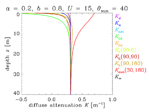
Figure 3 shows the K functions for a level surface and the Sun at the zenith, rather than at 40 deg. Again, the irradiance K functions are almost unchanged. However, the radiance function now corresponds to looking straight upward into the Sun’s direct beam. Thus now looks very similar to in the previous figures. Similarly, now looks much like in the previous figures. This is because moving the Sun from 40 deg in air (28 deg in water) to the zenith gives almost the same scattering angle relation to the Sun’s direct beam as had in the previous figures.
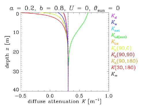
Figure 4 shows K functions for “highly absorbing” water: the absorption coefficient was , and the scattering coefficient was , so that the albedo of single scattering was . These values correspond roughly to what might be found at red wavelengths, where absorption by the water itself usually dominates the IOPs. Other conditions were the same as for Fig. 1.
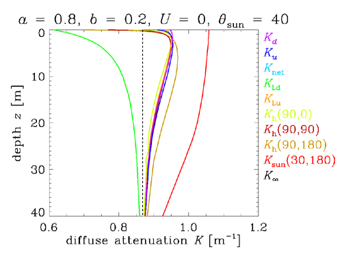
Comparing Figs. 1 and 4, we note that
- The rate of approach to the asymptotic value depends on the IOPs. In highly scattering water, the approach to is much faster than in highly absorbing water. This is because the near-surface radiance distribution must be “redistributed” by multiple scattering into the shape of the asymptotic radiance distribution in order for the K’s to approach . The more scattering, the faster the initial ray directions are changed by multiple scattering into their asymptotic distribution, which depends only in the IOPs.
Comparing Figs. 1 and 4 also shows that the K’s have changed greatly because of the change in IOPs, which is what is desired in any AOP. For the highly absorbing water, .
Beam Attenuation vs Diffuse Attenuation
The distinction between beam and diffuse attenuation is important. The beam attenuation coefficient c is defined in terms of the radiant power lost from a collimated beam of light. The downwelling diffuse attenuation function , for example, is defined in terms of the decrease with depth of the downwelling irradiance , which comprises light heading in all downward directions (a diffuse, or uncollimated, radiance distribution). In the above simulations, at all depths, but all K functions except the near-surface in the high absorption case are less than c. Radiative transfer theory shows (e.g., Light and Water (1994) Eq. 5.71) that in general , where is the mean cosine of the downwelling radiance. These inequalities are seen to hold true in the above simulations.
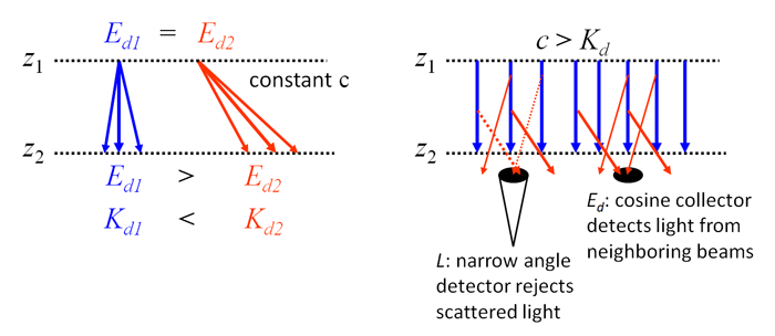
The left panel of Fig. 5 illustrates two different radiance distributions. The first, shown in blue, is directed more toward the nadir, and the second, shown in red, has a greater angle from the nadir. Even if the downwelling plane irradiances from both distributions are equal at depth , , they will not be equal at depth . The reason is that the red rays travel a greater distance in going from depth to . More energy will be lost to absorption from the red rays than from the blue rays because the path length of the red rays through the water is greater. Thus , which is equivalent to . In both cases, the beam attentuation is the same and does not depend on the depth if the water is homogeneous. Beam is an IOP and does not depend on the radiance distribution, whereas the AOP depends on the angular distribution of the radiance.
The right panel of the Figure shows why beam attenuation is always greater than diffuse attenuation . The blue arrows represent the rays of a collimated radiance in the nadir direction (). At the light propagates downward, some of the radiance will be scattered out of the beam at a particular horizontal location, as illustrated by the red arrows. A narrow-field-of-view radiance meter looking upward (measuring ) will detect the radiance that is transmitted from depth to with only small-angle scattering (scattering at angles less that the FOV; there will also be some loss to absorption). This detector will not detect radiance scattered from “neighboring” beams, which is illustrated by the dotted red arrows, because these rays are in directions outside the instrument FOV. The difference in and determines the beam attenuation averaged over the water column from to via
Now consider a plane irradiance detector measuring . This detector receives light from the beam directly above it, as did the detector, but it also receives some of the light scattered out of neighboring beams that would otherwise miss the detector. That is to say, part of the energy lost from one beam can be replaced by light scattered from nearby beams if the detector has a wide FOV. Thus the decrease in going from depth to , which determines , will be relatively less than the change in the radiances over the same distance, which determine . In other words, . only in the idealized case of a perfectly collimated downward radiance (such as the Sun at the zenith in a black sky) in water with no scattering and no internal sources.
The Effect of Inelastic Scattering on K Functions
HydroLight was next used to simulate a homogeneous Case 1 water body with a chlorophyll concentration of . As for Figs. 1 and 4, the Sun was at 40 deg and the surface was level. Figure 6 plots several quantities as a function of wavelength at 10 m depth for this simulation. We see that between 300 and about 600 nm, the various functions are very similar and proportional to the total (including water) absorption coefficient . However, beyond 600 nm the K functions differ from each other, and they are all much different from a. The reason for this behavior is inelastic scattering.
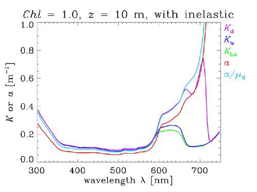
At the near-UV to blue to green wavelengths below 600 nm, most of the radiance at 10 m depth (for these IOPs) comes from sunlight being transmitted through the upper 10 m of the water column. Above about 600 nm, absorption by the water itself has removed most of the sunlight. For example, at 700 nm where , we expect roughly of the surface light to reach 10 m. However, Raman scatter and CDOM fluorescence inelastically scatter light from shorter wavelengths, where sunlight is present, into the red wavelengths, and thus create additional red light at 10 m. Thus, beyond 600 nm, the various radiances and irradiances no longer decrease with depth in a simple exponential fashion. Note that tracks a longer than do and . This is because continues to collect whatever downwelling sunlight remains, and thus the inelastic contribution to is not noticeable until the chlorophyll fluorescence contribution begins near 670 nm. and
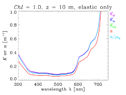
It is easy to verify that the peculiar behavior of the K functions beyond 600 nm is due to inelastic scatter. The HydroLight run was repeated with Raman scatter and CDOM and chlorophyll fluorescence “turned off.” Figure 7 shows the results. Now, the K functions all track the absorption nicely at all wavelengths.
As seen in these figures, radiative transfer theory shows that K functions are very “absorption like,” meaning that the K functions are strongly correlated with the total absorption coefficient when inelastic scatter effects are negligible. For , the approximate relation gives close agreement between the exact (computed by HydroLight) and the value estimated from the absorption coefficient and the downwelling mean cosine of the radiance distribution, which was also obtained from the HydroLight simulation.
These few simulations are enough to establish the salient features of diffuse attenuation functions. Their use has a venerable history in optical oceanography. Smith and Baker (1978) listed some of their virtues:
- The K’s are defined as ratios and therefore do not require absolute radiometric measurements.
- The K’s are strongly correlated with phytoplankton chlorophyll concentration (via the absorption coefficient) in Case 1 waters. Thus they provide a connection between biology and optics.
- About 90% of the diffusely reflected light from a water body comes from a surface layer of water of depth , which is called the “penetration depth.” Thus has implications for remote sensing.
- Radiative transfer theory provides several useful relations between the K’s and other quantities of interest, such as the absorption and beam attenuation coefficients and other AOP’s.
Gordon’s Normalization of
As seen above, does have some dependence on the Sun location and sky conditions, even though the dependence is weak. Gordon (1989) developed a simple way to normalize measured values. His normalization for all practical purposes removes the effects of the sea state and incident sky radiance distribution from , so that the normalized can be regarded as an IOP. The theory behind the normalization is given in his paper; the mechanics of the normalizing process are as follows.
Let be the irradiance incident onto the sea surface due to the Sun’s direct beam, and let be the irradiance due to diffuse background sky radiance. Then the fraction f of the direct sunlight in the incident irradiance that is transmitted through the surface into the water is
Here t(Sun) and t(sky) are respectively the fractions of the direct beam and of the diffuse irradiance transmitted through the surface; these quantities can be computed using methods described in Light and Water (1994) Chapter 4 [where they are denoted by ]. However, if the solar zenith angle in air, , is less than 45 degrees , then . If the sky radiance distribution is roughly uniform (as it is for a clear sky), then . In this case, we can accurately estimate f from measurements made just above the sea surface:
The Sun and sky irradiances are easily obtained from an instrument on the deck of a ship. When both direct and diffuse light fall onto the instrument, it records . When the direct solar beam is blocked, the instrument records . (Advanced technology is not required here: just hold your hat so that its shadow falls on the instrument.)
Next compute the nadir angle of the transmitted solar beam in water, , using Snell’s law:
Finally, compute the quantity
This value of is valid for flat or rough sea surfaces as long as . For larger values of , or for an overcast sky, a correction must be applied to to account for surface wave effects on the transmitted light; the correction factors are given in Gordon (1989, his Fig. 6). Gordon’s normalization then consists simply of dividing the measured by :
Physically, is a function (essentially ) that reduces values to the values that would be measured if the Sun were at the zenith, if the sea surface were level, and if the sky were black (i.e., if there were no atmosphere). The zenith-sun, level-surface, black-sky case is the only physical situation for which . In other words, normalization by removes the influence of incident lighting and sea state on . The same normalization can be applied to depth-averaged values of .
It is recommended that experimentalists routinely make the simple measurements necessary to determine , because normalization of enhances its value in the recovery of IOP’s from irradiance measurements.
 See comments posted for this page and leave your own.