Page updated:
March 13, 2021
Author: Curtis Mobley
View PDF
Theory of Fluorescence and Phosphorescence
Luminescence refers to the emission of light by processes other than thermal emission, which is called incandescence. There are many types of luminescence: fluorescence, phosphorescence, chemiluminescence, triboluminescence, radioluminescence, and so on. The luminescent processes that are of interest in oceanography are fluorescence, phosphorescence, and bioluminescence, which is a form of chemiluminescence.
When light is absorbed by a molecule, one of three things can happen:
- 1.
- the energy is used for photochemisty, e.g. for photosynthesis in a chlorophyll molecule;
- 2.
- the energy goes into vibrational modes of the molecule, i.e. into heat; or
- 3.
- the energy is re-emitted as light via fluorescence of phosphorescence.
This page develops the general theory needed to include fluorescence by chlorophyll and colored dissolved organic matter (CDOM) in radiative transfer calculations. Specific implementations of the general theory for chlorophyll and CDOM fluorescence are given on the next two pages.
The Physics of Fluorescence and Phosphorescence
The Pauli Exclusion Principle is one of the foundations of quantum mechanics. It states that no two fermions in an atom or molecule can have the same set of quantum numbers. Fermions are particles with an intrinsic angular momentum or “spin” that is a half-integer multiple of , where is Planck’s constant. Electrons are fermions with an angular momentum of and are called “spin 1/2” fermions. Thus for our purposes, the Pauli Exclusion Principle says that two electrons in the same atomic or molecular orbital must have opposite spins, which are called “up” and “down.” (The labels “up” and “down” historically refer to orientations of the angular momentum vector relative the direction of an external magnetic field. “Up” and “down” correspond to spin quantum numbers of s = +1/2 and -1/2. For more on the terminology of quantum numbers, orbitals, etc. see The Physics of Absorption.)
A singlet state of a molecule is one in which all electrons are paired in up and down pairs. A triplet state is one in which one set of two electrons in different orbitals have the same orientation, up-up or down-down. Figure 1 illustrates the idea. (Again, the terminology is historical and relates to the number of lines seen in a spectrum for molecules that are not spherically symmetric or when when a molecule is placed in a magnetic field, which splits the energy states. There is also a doublet state corresponding to one un-paired electron, but it does not concern us here.)
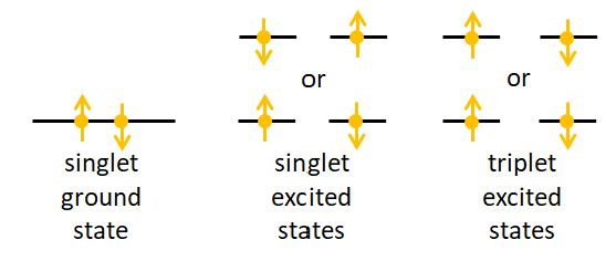
Figure 2 is a Jablonski diagram of energy states in a molecule. (The guy’s name is properly spelled Jabłoński. The Polish “J” is like the English “Y”; the L with a line through it is like the “W” in water, and the accented N is like the Cyrillic “H” in the Russian word“HeT,” or Nyet in English. So Jabłoński is pronounced something like YabWoNYski with English spelling; the accent is on the second syllable. He is one of those unfortunate souls who, like Khrushchev and Gengis Kahn, are forever doomed to have their names mispronounced by English speakers.) Such diagrams group the energy levels vertically and the spin states horizontally. The black lines represents the energy levels; the thick lines labeled and are the electronic levels, and the thinner lines are vibrational levels. The gold dots with arrows represent electrons in either up or down angular momentum states.
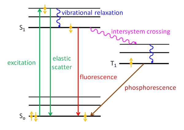
Now suppose that one of the electrons of an electron pair, say the down electron, in the ground state of a molecule absorbs a photon. The energy of the photon excites the electron to a higher energy level as shown by the upward green arrow. The time scale for this excitation is on the order of . The electron spin is still down in the excited energy level. One thing that can happen is that the electron almost immediately drops back to the ground state with emission of a photon with the same wavelength as the excitation photon. This is elastic scattering and is represented by the green downward arrow in the figure. This process is so fast that the excited electron “remembers” the direction of the incident photon, and the direction of the emitted/scattered photon depends on the direction of the incident photon; i.e., the scattering is not isotropic.
Another thing that can happen is that part of the energy of the excited electron is given up to other vibrational modes (i.e., to heat), so that the electron drops to a lower energy level of the excited state. This is indicated by the blue wiggly line labeled “vibrational relaxation” in Fig. 2. This loss of energy is called a “radiationless transition” because it does not involve the emission of a photon. The time scale for vibrational relaxation is -. The electron may stay in the excited state for a while, but if the electron is still in the down state, i.e. it is in a singlet state, it can drop back to the ground level by emission of a photon of lower energy (longer wavelength) than the exciting photon. The time scale for this is of order -. The ground state then once again contains an up-down pair of electrons. This is fluorescence and is shown by the red downward arrow in the figure. The processes of vibrational relaxation and fluorescence emission take so long that the electron has “forgotten” the direction of the incident photon, and the emitted photon is equally likely to be in any direction; i.e., the emission of fluoresced light is isotropic.
An electron cannot just simply “flip” from a down to an up state, which would violate the law of conservation of angular momentum. Such a flip is therefore a “forbidden transition” in quantum mechanics terminology. However, in quantum mechanics, “forbidden” does not mean “do not ever do something,” just “do not do it vary often.” So a third thing that can happen is that the down electron sitting in the state can exchange some angular momentum with the orbital angular momentum of the molecule via what is called “spin-orbit coupling.” The electron can then flip to an up state. This is another radiationless transition and is called an “intersystem crossing” and is shown in purple in Fig. 2. The time scale for intersystem crossing is on the order of -. The electron can also undergo further vibrational relaxation in the triplet state. This up electron is no longer paired with the up electron that was left in the ground state; it is in an excited triplet state, which is labeled by in figure. The energy level of the first excited triplet state is usually lower than for the first excited singlet state because the electrons are further apart, which makes their Coulomb repulsion less. This up electron cannot drop back to the ground state because the result would give two up electrons in the ground state, which violates the Pauli Exclusion Principle; this is another forbidden transition. Therefore the up electron in the state must wait for another chance for spin-orbit coupling, which can flip its spin to down. This takes a long time (on the atomic scale), so the state is called “metastable.” That down electron can then drop into the down-electron spot in the ground level, which is again paired with the up electron in the ground state. This process is phosphorescence and can take from to as long as . The emitted light is again isotropic because of the long time between absorption and re-emission.
In summary, fluorescence is a transition from an excited singlet state to the ground singlet state, and phosporescence is a transition from an excited triplet state to the ground singlet state. There are other pathways to fluorescence. For example, the original absorbed photon could excite the ground state electron to the state (second excited singlet state), which might then do a radiationless transfer of energy to an overlapping vibrational level of the orbital; this is called “internal conversion” (internal within a singlet state), and the time scale is -. The electron can then vibrationally relax to the level, and then fluoresce, and so on. It should also be noted that there are many vibrational energy levels in each of the electronic levels illustrated in Fig. 2, and transitions can occur between any of these. This gives a spread of energies of the emitted emitted photons, i.e, a spread of wavelengths. See the related discussion on the The Physics of Absorption page.
The time scales of elastic scattering, and of Raman Scattering, are so short, or less, that they are called “scattering.” Fluorescence and phosphorescence are, however, clearly absorption followed much later by the emission of a new photon that is uncorrelated with the absorbed photon. However, for the purposes of most optical oceanography, and for solution of the time-independent radiative transfer equation in particular, fluorescence and phosphorescence can be regarded as “inelastic scattering” and treated with the same mathematical formalism as that used for Raman scattering. This is the case for “solar-stimulated” chlorophyll and CDOM fluorescence.
However, measuring the time dependence of fluorescence emission at time scales of to gives information about the internal details of the energy transfers within the molecule. Indeed, the quantum efficiency of chlorophyll fluorescence is dermined by measuring the decay of chlorophyll fluorescence (on a time scale of order 10 ns) excited by an extremely short light pulse (or order 1 ns). Thus time-resolved measurements of chlorophyll fluorescence give information about the photosystems responsible for photosynthesis and the effect of environmental stresses (pH, light adaptation, etc) on those systems. That requires a much more complicated modeling of fluorescence than what is discussed here. See Falkowski et al. (2017) for an overview of time-resolved chlorophyll fluorescence measurements.
Incorporation of fluorescence into time-independent radiative transfer theory
The quantities needed to compute fluorescence contributions to the radiance are
- the fluorescence scattering coefficient , with units of ,
- the fluorescence wavelength redistribution function , with units of , and
- the fluorescence scattering phase function , with units of .
The subscript “F” indicates fluorescence; it will be replaced on the next pages by “C” for chlorophyll or “Y” for yellow matter (and it was “R” in the discussion of Raman scatter, which uses the same mathematical formalism). The amount of fluorescing material, e.g. the amount of chlorophyll or CDOM, in general depends on depth, whereas the wavelength redistribution function is determined only by the type of fluorescing material. The phase function is isotropic. It is thus reasonable to place the depth dependence of the fluorescence in the scattering coefficient.
Multiplied together, these functions give the volume inelastic scattering function for fluorescence :
| (1) |
This function is used as a source function in the scalar radiative transfer equation (See Eq. 3 of The Scalar Radiative Transfer Equation):
This is the same set of quantities required to describe Raman scatter. Of course, the functional forms and magnitudes of these quantities will be different for Raman scatter, chlorophyll fluorescence, and CDOM fluorescence.
It must be remembered that radiative transfer theory is formulated in terms of energy. For fluorescence, the quantity of interest in computing radiance via Eq. (2) is how much energy is emitted by fluorescence compared to how much energy is absorbed. However, the folks who study fluorescence usually work in quantum units, i.e., how many photons are emitted as fluorescence compared to how many photons are absorbed. Accordingly, the spectral fluorescence quantum efficiency function is defined as
The numerator of this function must be multiplied by , and the denominator by , to convert the photon counts to energy. The result is that
| (3) |
Another quantity often seen in the literature is the non-dimensional quantum efficiency (or quantum yield) of fluorescence, which is defined by
is obtained from by
| (4) |
A paper on chlorophyll fluorescence may discuss other quantum efficiencies, namely a quantum efficiency for photosynthesis and a quantum efficiency for heating . The quantum efficiency for photosynthesis is the ratio of photons whose energy goes into photosynthesis to the number of photons absorbed, and similarly for the number whose energy stays in vibrational modes (i.e., heat). From the opening comments of this page it follows that . Typical upper-ocean numbers as measured by Falkowski et al. (2017) are , , and .
Comments on Terminology
It might appear that or is the fluorescence “excitation-emission” (Ex-Em) function or matrix that is commonly seen in papers (e.g., Fig. 5 of the CDOM fluorescence page). However, these are different quantities. is a fluorescence efficiency that measures how many quanta are emitted per quanta absorbed. Ex-Em functions are measurements of the number of emitted quanta (e.g., as counts per second) without regard for how many quanta are absorbed. In addition, the factor of that converts to shifts the location of maxima in the functions because different wavelengths correspond to different numbers of quanta for the same energy. Thus and Ex-Em spectra are qualitatively similar in appearance, but quantitative comparison is difficult. In addition, Ex-Em spectra are often presented as normalized values, which makes quantitative comparison impossible. Relative excitation and emission values have many uses, but the radiative transfer equation requires a calibrated function in units of 1/nm.
I have called the “spectral fluorescence quantum efficiency function”, which comes from Hawes (1992). This is in fact the only study I have found that measures this function (for CDOM fluorescence) in a calibrated form suitable for radiative transfer theory. I called the energy equivalent the “wavelength redistribution function” in Light and Water because it tells how energy at the excitation wavelengths is redistributed to the emission wavelengths , but maybe the “spectral fluorescence energy efficiency function” would be a better name. Gordon (1979) calls a nondimensional function equivalent to the “quantum efficiency.” Gordon calls my “volume inelastic scattering function for fluorescence” the “volume fluorescence function,” and he calls
the “coefficient of fluorescence.”
I have talked to a couple of researchers in fluorescence about the need for calibrated excitation-emission functions in radiative transfer theory, i.e. my or , but the response has been that they do not need calibrated functions for their applications, so they do not attempt to measure them. I will leave it at that and define quantities as needed; I hope that my definitions are clear, even if the terminology is sometimes non-standard.
 See comments posted for this page and leave your own.