Page updated:
March 6, 2021
Author: Curtis Mobley
View PDF
Geometrical Radiometry
Curtis Mobley and Kenneth Voss contributed to this page.
By housing one or more radiant energy detectors in watertight assemblies and by appropriately channeling the direction of the radiant energy arriving at the detector, we can measure the flow of radiant energy as a function of direction at any location within a water body. By adding appropriate filters to the instrument, we can also measure the wavelength dependence and state of polarization of the light field. From such measurements we can develop precise descriptions of radiative transfer in natural waters. Thus we are led to the science of geometrical radiometry, the union of Euclidean geometry and radiometry.
We first define radiance, the fundamental quantity that describes light in radiometric terms. We then define various irradiances and other quantities that are derivable from the radiance, and which are often easier to measure and of more relevance to a particular problem.
Radiance
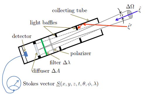
Figure 1 shows the design of a Gershun tube radiometer. A circular hole at one end of the housing or collecting tube and a system of internal light baffles allows the detection of light that enters the hole only at angles of or less (measured from the axis of the tube). Angle is the field of view (FOV) half angle. The blue arrow in the figure represents light entering the tube within the field of view. Light entering the tube at angles larger than , represented by the red arrow in the figure, is blocked by the baffles or absorbed by the inner walls of the tube and is not detected. In most instruments, is around 5 deg (at most 10 deg). The solid angle seen by the detector is .
If the state of polarization is of interest, a polarizing filter is placed in the tube so that the light passes first through the polarizer. This filter will be chosen to measure the desired component of the polarization, e.g, horizontal or vertical plane polarization, or left or right circular polarization. In practice, a sequence of measurements must be made to determine the four components of the Stokes vector; see the page on Polarization for further discussion.
A wavelength filter is normally used to select a narrow band of wavelengths. In modern instruments this is usually an interference filter that passes light of some bandwidth centered at the nominal wavelength . In the early days of optical oceanography, the filter was often a gelatine filter than passed certain wavelengths and absorbed others. In most instruments is around 10 nm (at most, 20 nm), but can be only a few nanometers for hyperspectral instruments.
Finally, the light, which is still well collimated after passing through the polarizer and wavelength filter, passes through a translucent diffuser of collection area . The diffuser makes the light field spatially homogeneous in the region near the detector, so that it is necessary to sample only a part of the internal light field in order to measure the total energy entering the instrument. To the accuracy with which , the solid angle of the hole as seen by any point on the diffuser surface is the same.
In order to measure an entire spectrum, an instrument may have a rotating wheel holding many different wavelength filters, or it may use a prism to spread the different wavelengths out along a CCD array. Similarly, an instrument may have a rotating wheel holding different polarization filters, so as to obtain all components of the Stokes vector by a sequence of measurements as the wheel rotates. These engineering details do not concern us in the present discussion, but they are of great importance in the construction of actual instruments.
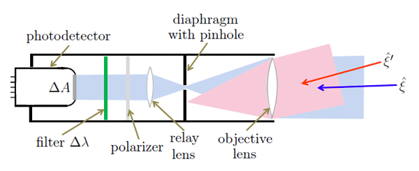
The instrument design of Fig. 1 traces back to the Russian physicist and pioneer of optical oceanography A. A. Gershun in the 1930s. Instruments implementing variants of his design are still in production. Figure 2 shows a more modern design that uses lenses and a pinhole in a diaphragm to select the directions of light propagation that can be detected. As shown, an objective lens focuses the incoming light onto an opaque diaphragm, which contains a small hole on the optical axis. Light propagating in a narrow range of directions (the FOV) will pass through the pinhole and be detected. This is illustrated by the blue arrow and the bluish shading in the figure. Light propagating in directions outside the FOV will not pass through the pinhole. This light is illustrated by the red arrow and the reddish shading. The light that does pass through the pinhole is then collimated by a relay lens and directed towards a detector with detecting area . Again, polarizers or wavelength filters can be part of the design. As drawn, the polarizer is placed after the two lenses. This layout is acceptable for glass lenses, which do not significantly affect the state of polarization. If the lenses are made of plastic or another material that alters the state of polarization, then the polarizer needs to be in front of the objective lens. The FOV and corresponding solid angle seen by the detector are determined by the lens and pinhole geometry.
The designs of both Figs. 1 and 2 are termed “well collimated radiometers” because they detect light propagating in only a narrow set of nearly collimated directions.
If the instrument is pointing in the direction, it collects light traveling in a set of directions of solid angle centered on direction . We assume that the instrument is small compared to the scale of spatial (positional) changes in the light field, so that we can think of the instrument as being located at a point within a water body. Suitable calibration of the current or voltage output of the detector gives the amount of radiant energy entering the instrument during a time interval centered on the time . For simplicity, consider the total radiance without regard for the state of polarization (that is, remove the polarizer in either of the instrument designs); this is the first component of the Stokes vector and is commonly called the radiance. An operational definition of the unpolarized spectral radiance is then
| (1) |
In practice the intervals , , , and are taken small enough to get a useful resolution of over the various parameter domains, but not so small as to encounter diffraction effects or fluctuations from photon shot noise at low light levels. Typical values are to (depending on whether one wishes an “instantaneous” measurement or wishes to average out sea surface wave effects), , to 0.1 sr, and 1 to 10 nm. In radiative transfer theory, the direction always denotes the direction of propagation of the light. The viewing direction, which is the direction an instrument is pointed to detect , is then .
In the conceptual limit of infinitesimal parameter intervals, the spectral radiance is given by
| (2) |
This definition of radiance is convenient for the mathematical development of radiative transfer theory. The operational definition is what is used for actual measurements.
Spectral radiance is the fundamental radiometric quantity of interest in hydrologic optics. It specifies the spatial (), temporal (), directional (), and wavelength () structure of the light field. As we shall see, all other radiometric quantities can be derived from L.
Although radiance is an extremely useful concept and is adequate for most needs of optical oceanography, it is an approximation to the exact description of light in terms of electric and magnetic fields. We therefore anticipate that there are situations for which radiance fails to give an adequate description of the light field. When that happens, we must resort to Maxwell’s Equations and compute the electric and magnetic fields themselves. Some of the Limitations of Radiance are discussed in Level 2 of this chapter. Moreover, both because of instrumental difficulties and because such detailed directional information often is not needed for specific applications, the most commonly measured radiometric quantities are various irradiances.
Plane Irradiance
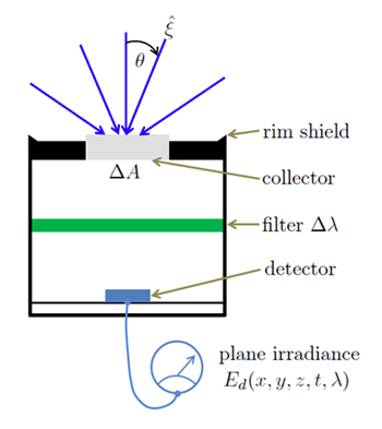
If the collecting tube is removed from the instrument of Fig. 1, then light from an entire hemisphere of directions can reach the detector, as illustrated in Fig. 3. Such an instrument, when pointed “straight up” (in the direction) so as to detect light headed downward (all in ) measures the spectral downwelling plane irradiance :
| (3) |
Implicit in this definition is the assumption that each point of the collector surface is equally sensitive to light incident onto the surface from any angle. If this is the case, however, the collector as a whole is not equally sensitive to light headed in all downward directions. Imagine a collimated beam of light headed straight downward (e.g. from the sun straight overhead). This beam, assumed to be larger than the collector surface, sees the full area of the collector surface. However, the same large beam traveling at an angle relative to the instrument axis sees a collector surface of effective area (the area as projected onto a plane perpendicular to the beam direction). Otherwise identical collimated light beams therefore generate detector responses that are proportional to the cosines of the incident directions. Such instruments are called cosine collectors.
The cosine law for irradiance is simply the statement that a collimated beam of light intercepting a plane surface produces an irradiance that is proportional to the cosine of the angle between the incident directions and the normal to the collector surface.
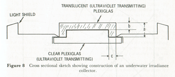
There are subtleties in the construction of instruments that require a cosine response. No real material used for the collector actually obeys the requirement that every point of the material surface be equally efficient at collecting energy from any direction. In practice, surfaces often look a bit “shiny” near grazing angles ( near 90 deg). Thus more of the incident energy is reflected by the collector surface at large values. To correct for this less efficient energy collection at large , the collector itself often extends a small distance above the instrument housing, as seen in Fig. 3. The vertical walls of this “button” then receive the light at more nearly normal directions to the vertical edge of the collector. However, that vertical collector side would collect light propagating at = 90 deg, which should give no response according to the cosine law. To block light incident when is within a few degrees of 90, the rim of the housing has a low “wall” that blocks light at very near 90 deg. An actual implementation of this idea is seen in Fig. 4. Modern instruments with similar designs achieve an in-water cosine response to within a percent or two.
Another very important issue with the construction an in-water cosine collector is that the reflective properties of collector materials such as glass, plastic, or Spectralon are much different in water than in air. This is because of the differences in the collector-air and collector-water indices of refraction. For example, Spectralon, which is often used in optical instruments, has a refractive index of 1.35. This is very close to that of water, which is about 1.33 (with some wavelength variation in each). Air has a refractive index of almost exactly 1. At normal incidence the reflectance of an air-Spectralon surface is
For a water-Spectralon surface the corresponding reflectance is only 0.00006. Thus more light gets “into” the collector made of Spectralon when the instrument is in water than when it is in air. Conversely, more of the collected light can escape “back out” from the Spectralon collector in water than in air. Therefore different fractions of the incident energy are collected and reach the detector for the same instrument when used in air and in water. This difference is called the immersion effect.
The consequence of these observations is that if a sensor is to be used in water, the design (such as seen in Fig. 4 ) must be such that the sensor has a cosine response in water, and the sensor calibration must account for the immersion effect. These matters are crucial to the design of irradiance sensors, but the details can be left to the optical engineers.
Since the instrument of Fig. 3 collects light traveling in all downward directions, but with detector’s surface area weighted by the cosine of the light’s incident angle , the instrument is in essence integrating over all incident directions in the hemisphere seen by the sensor. The spectral downwelling plane irradiance is therefore related to the spectral radiance by
If the same instrument is oriented downward, so as to detect light heading upward, then the quantity being measured is the spectral upwelling plane irradiance :
| (5) |
Note that it is necessary to take the absolute value of cos in Eq. (5) because, with our choice of coordinates, for in . The absolute value is superfluous in Eq. (4).
Scalar Irradiance
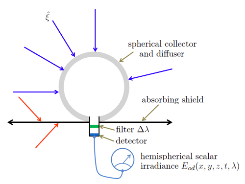
Now consider an instrument that is designed to be equally sensitive to all light headed in the downward direction. Such an instrument is shown in Fig. 5. The spherical shape of the collector and diffuser insures that the instrument is equally sensitive to light from any direction. If each point on the diffuser surface behaves like a cosine collector, then the effective area of the collector is , where is the radius of the diffuser. In addition, the radiance distribution in the hollow interior of the collector is isotropic, so that only a small part of the interior light field needs to be measured. The large shield blocks upward-traveling light. In principle, this shield extends to infinity in all directions, but in reality may be only a few centimeters in diameter. The upper surface of the shield is assumed to be completely absorbing, so that it cannot reflect downward traveling light back upward onto the collector. These cases are illustrated by the red arrows in the figure. This instrument, when oriented upward as shown in Fig. 5, measures the spectral downwelling scalar irradiance , which is related to the spectral radiance by
If the instrument of Fig. 5 is inverted, so as to collect only upward traveling light, then it measures the spectral upwelling scalar irradiance . If this shield is removed, light traveling in all directions is collected. The quantity then measured is the spectral total scalar irradiance , which is related to the radiance by
Other possible instrument designs are discussed in Hojerslev (1975). However, the three basic types shown above are sufficient for most of the needs of hydrologic optics. Such instruments are commercially available.
Vector Irradiance
The spectral vector irradiance is defined as
| (8) |
Recalling that the vertical component of is just , we can write the vertical component of the vector irradiance as
In developing Eq. (9), we have noted that in and in . The quantity is called the net downward irradiance. This net downward irradiance often is often called the “vector” irradiance, although strictly speaking it is only the vertical component of the vector irradiance. If the radiance distribution is horizontally homogeneous, the horizontal components of the vector irradiance are zero.
Example: Irradiances of an isotropic radiance
distribution
Consider an isotropic, or directionally uniform, radiance distribution: for all in . Then by Eq. (4), the downward plane irradiance is
In the last equation, carries units of steradian from the integration over solid angle; thus has units of irradiance when has units of radiance. Likewise, , so that the net downward irradiance is zero. The scalar irradiance is given by Eq. 6
In the same manner we find , so that the total scalar irradiance .
Photosynthetically Available Radiation
Photosynthesis is a quantum process. That is to say, it is the number of photons absorbed rather than their total energy that is relevant to the chemical transformations. This is because a photon of, say, wavelength 400 nm, if absorbed by a cholorphyll molecule, induces the same chemical change as does a less energetic photon of wavelength 500 nm. (However, photons of different wavelengths are not equally likely to be absorbed.) Only a part of the photon’s energy goes into photosynthesis; the excess appears as heat or is re-radiated. Moreover, chlorophyll is equally able to absorb light regardless of the light’s direction of travel.
Now recall that the spectral total scalar irradiance is the total radiant power per square meter at wavelength coursing through point owing to light traveling in all directions. The number of photons generating is . Therefore, in studies of phytoplankton biology, a useful measure of the underwater light field is the photosynthetically available radiation, PAR or , which is defined by
| (10) |
Note that PAR is by definition a broadband quantity. Bio-optical literature often states PAR values in units of or . Recall from the table of derived units that one einstein is one mole of photons ().
Morel and Smith (1974) found that over a wide variety of water types from very clear to turbid, the conversion factor for energy to photons varies by only about the value
PAR is usually estimated using only the visible wavelengths, 400-700 nm, although some investigators include near-ultraviolet wavelengths in the integral of Eq. (10). PAR is also sometimes estimated using rather than . This usually underestimates PAR by 30% or more because is always less than .
Instruments for the direct measurement of PAR, often called quanta meters, can be constructed along the lines of Fig. 5 by the incorporation of broadband wavelength filters. Such instruments are commercially available. Engineering details can be found in Jerlov and Nygård (1969) and in Kirk (1994), which also discusses PAR and photosynthesis in great detail.
Although PAR has a venerable history as a simple parameterization of available light in phytoplankton growth models, it should be noted that PAR is an imperfect measure of how light contributes to photosynthesis. This is because different species of phytoplankton, or even the same species under different environmental conditions, have different suites of pigments. Phytoplankton with different pigments absorb light differently as a function of wavelength. Thus phytoplankton with different pigments use the same with different efficiencies, thus giving one an advantage over the other. Recent ecosystem models therefore replace PAR by spectral scalar irradiance and also account for different pigments in different functional classes of phytoplankton. Such models can better simulate how light is utilized by different components of the ecosystem (e.g., Bissett et al. (1999); Fujii et al. (2007).
Intensity
Another family of radiometric quantities can be defined from the measurements employed in the operational definition of radiance. The spectral intensity I is defined as
| (11) |
or
In Eq. (12), is the surface of the collector that sees the solid angle , and is an element of area. The concept of intensity is useful in the radiometry of point light sources. We will use it in Chapter 3 in the definition of the volume scattering function.
Terminology and Notation
The adjective “spectral,” as in spectral radiance, as commonly used can mean either “as a function of wavelength” or “per unit wavelength interval.” Committees on international standards recommend an argument , e.g. , for the first meaning and a subscript , e.g. , for the second meaning (Meyer-Arendt (1968)). However, this subscript convention is seldom used in optical oceanography, perhaps because the symbols already are cluttered with subscripts. Most authors seem to write and consider it to mean radiance per unit wavelength interval, as a function of wavelength. The adjective spectral and argument are often omitted for brevity, although strictly speaking, a term without the adjective “spectral” refers to a quantity integrated or measured over a finite band of wavelengths, as in the computation of PAR in Eq. (10). Most radiative transfer theory assumes the energy to be monochromatic, i.e., radiance per unit wavelength interval at a particular wavelength. However, most measurements are made over a wavelength band of 1 to 20 nm, which complicates the comparison of theory and observation.
Spectral quantities are sometimes expressed in terms of a unit frequency interval rather than a unit wavelength interval. To establish the conversion, consider the radiant energy contained in a wavelength interval . The same amount of energy is contained in a corresponding frequency interval . Since an increase in wavelength () implies a decrease in frequency (), and vice versa, we can write
Using we then get
which is the desired connection between and , or between any other radiometric quantities. A wavelength interval therefore corresponds to a frequency interval of size
The wavenumber is also sometimes used (the value usually given in inverse centimeters, ). An analysis parallel to that just given yields
Since sampling times are generally long compared to the time () required for the light field in a water body to reach steady state after a change in the environment, time-independent radiative transfer theory is usually sufficient for hydrologic optics studies. In this case, the time is implicitly understood and the argument can be omitted. A notable exception to the use of time-independent radiative transfer theory occurs with the use of pulsed lasers to determine water depth or to detect underwater objects. In this application, the laser pulses last only for nanoseconds and time-dependent theory must be used.
Finally, time-averaged (over seconds to minutes) horizontal variations (on a scale of meters to kilometers) in the environment and in the optical properties of natural water bodies illuminated by the sun are usually much less than vertical variations. In that case, underwater light fields depend spatially only on the depth to a good approximation. Thus, for example, we often can refer to just “the radiance ” without generating confusion. An important exception of this situation occurs with artificial light sources, such as an underwater light or a laser being used for bathymetric mapping. In these cases the horizontal variations in the radiance can be large, and the three-dimensional spatial variations of the light field must be considered.
Although this web site uses the terminology and notation commonly seen in the current optical oceanographic literature, much published work uses a different nomenclature. Prior to the late 1970’s, different symbols were often employed for the radiometric concepts just defined. This historical notation is seen, for example, in the monumental treatise (Hydrologic Optics by Preisendorfer (1976). There is a Level 2 discussion of historical notation and of further subdivisions of radiometric concepts into field (energy falling onto a surface) vs. surface (energy emitted by a surface) quantities.
Much of the radiative transfer work in atmospheric, astrophysical, and biomedical optics, and in neutron transport theory, is relevant to hydrologic optics. However, to a considerable extent, these fields have developed independently and each has its own nomenclature. For example, in atmospheric and astrophysical optics, radiance is often called “intensity” or “specific intensity” and is given the symbol ; this use of “intensity” is not be confused with intensity as defined above. The classic text by van de Hulst (1957) uses “intensity” for irradiance. The letter “” often is used as the symbol for irradiance. The word “flux” is sometimes used to mean irradiance and is sometimes used to mean power. Those who use “flux” for power generally use “flux density” for irradiance. The ambiguity associated with “flux” can be avoided simply by using “power” or “irradiance,” as is appropriate. Matters are further complicated by the occasional misuse of photometric terms such as “brightness” and “luminance” for radiometric quantities; these matters are discussed in the Chapter on Photometry and Visibility.
 See comments posted for this page and leave your own.