Page updated:
October 28, 2020
Author: Curtis Mobley
View PDF
Reflectances
Various reflectances are probably the most commonly used apparent optical properties because they are fundamental to remote sensing of the oceans. In the early days of ocean color remote sensing, algorithms were developed to relate the irradiance reflectance to quantities such as absorption and backscatter coefficients and chlorophyll concentrations (e.g., Morel and Prieur, 1977; Gordon and Morel, 1983). More recently, the remote-sensing reflectance has become the AOP of choice for remote sensing of ocean properties (e.g., O’Reilly et al. (1998); Mobley et al. (2005)). This page considers each of these reflectances.
The Irradiance Reflectance
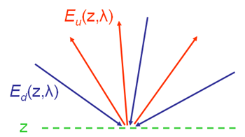
The spectral irradiance reflectance (or irradiance ratio), , is defined as the ratio of spectral upwelling to downwelling plane irradiances:
is thus a measure of how much of the radiance traveling in all downward directions is reflected upward into any direction, as measured by a cosine collector. This is illustrated in Fig. 1. Depth can be any depth within the water column, or in the air just above the sea surface.
Irradiance reflectance has the virtue that it can be measured by a single, uncalibrated, plane irradiance detector. The downwelling irradiance can be measured, and then the detector can be turned “upside down” to measure . The calibration factor needed to convert from detector units (voltage, current, or digital counts) to irradiance units () cancels out.
One of the pioneering papers on the use of spectra to obtain IOPs is Roesler and Perry (1995). They first developed a model for , where and are the total backscatter and absorption coefficients. These IOPs were then written as sums of contributions by water, phytoplankton, dissolved substances, and non-living particles (tripton). The resulting model was then forced to fit measured spectra, whereby the best fit determined the concentrations of the various components.
The Remote-Sensing Reflectance
The spectral remote-sensing reflectance is defined as
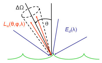
Here the depth argument of “in air” indicates that is evaluated just above the water surface using the water-leaving radiance and in the air. Water-leaving radiance refers to downwelling light that has entered the water body from the air, been scattered into upward directions within the water, and then been transmitted through the water surface back into the air. The remote-sensing reflectance is thus a measure of how much of the downwelling radiance that is incident onto the water surface in any direction (as measured by a plane irradiance sensor) is eventually returned through the surface into a small solid angle centered on a particular direction , as illustrated in Fig. 22.
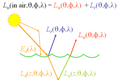
Although is often computed for nadir-viewing directions only, in actual remote sensing it is usually an off-nadir direction that is being observed by an airborne or satellite remote sensor. As shown next, has the virtue that it is less sensitive than to environmental conditions such as Sun zenith angle or sky conditions. This is the reason that has replaced for remote sensing. However, determination of is more difficult than . First, the measurements of and require different sensors, which must be accurately calibrated. Second, the water leaving radiance cannot be measured directly. Only the total upwelling radiance above the surface can be measured. This is the sum of the water-leaving radiance and the downward Sun and sky radiance that is reflected upward by the sea surface, , as illustrated in Fig. 3. therefore must be estimated either from a measurement of the total upwelling radiance made above the sea surface, or from a measurement of made at some distance below the sea surface and extrapolated upward through the surface. Each of these estimation methodologies has arguments for and against its use (e.g., Mobley (1999); Toole et al. (2000)).
Dependence of and on IOPs and Environmental Conditions
To illustrate the dependence of and on IOPs and external environmental conditions, the HydroLight radiative transfer numerical model was run using an IOP model for Case 1 waters with chlorophyll concentrations of , and . For each chlorophyll concentration, runs were made for three sets of sky conditions: (1) a level sea surface (windspeed ) and the Sun at the zenith (Sun = 0) in a clear sky; (2) a rough sea surface with a wind speed of and the Sun at a 50 deg zenith angle (Sun = 50) in a clear sky; (3) a wind speed of and a heavily overcast sky (overcast) for which the Sun’s location cannot be discerned.
Figure 4 shows the resulting spectra at depth , which is in the water just below the mean sea surface. This is the quantity most often used to develop remote-sensing algorithms relating to IOPs or chlorophyll concentrations. The curves for the different chlorophyll concentrations group together, showing that the shapes of the spectra are determined primarily by the different IOPs associated with the different chlorophyll concentrations. However, there is also a significant effect of the sky conditions on the spectra within each of the three chlorophyll groups.
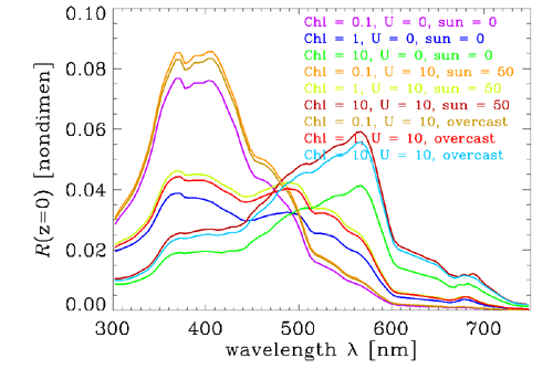
Figure 5 shows the nadir-viewing spectra for the same set of HydroLight runs. The three chlorophyll groups are similar in shape to the corresponding spectra, but there is much less variability in the spectra due to the external environmental conditions. is thus a better AOP than is , because is less sensitive to the sky conditions while remaining very sensitive to the different IOPs corresponding to the different chlorophyll concentrations.
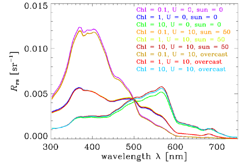
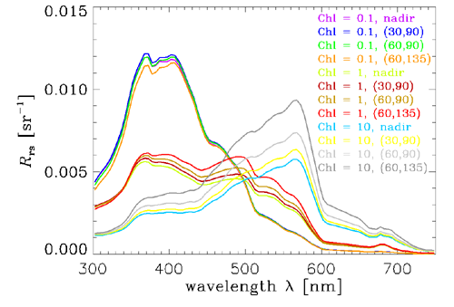
Figure 6 shows the spectra for nadir vs. various off-nadir viewing directions. Azimuthal angle corresponds to looking at right angles to the Sun’s azimuthal direction, and is looking half-way between normal to the Sun and away from the Sun. This range of values is what is usually observed in remote sensing to avoid Sun glint from the sea surface. At the lowest chlorophyll concentration, there is not much difference in the spectra for the different viewing directions. However, the differences increase with increasing chlorophyll concentration, and are quite significant for the curves when . These differences in off-nadir directions for different chlorophyll values are a consequence of the changes in shape and relative importance of the scattering phase functions for the small and large chlorophyll-bearing particles versus that of water as the chlorophyll concentration increases.
As Figs. 5 and 6 show, is much more sensitive to water IOPs than to external environmental conditions and viewing direction. However, still does depend somewhat on solar zenith angle (Fig. 5) and viewing direction (Fig. 6). An even better AOP would be obtained if these remaining dependencies can be removed. The resulting AOP is called the exact normalized water-leaving reflectance, denoted by . This reflectance is based on the concept of the normalized water-leaving radiance, which is defined to be “...the radiance that could be measured by a nadir-viewing instrument, if the Sun were at the zenith in the absence of any atmospheric loss, and when the Earth is at its mean distance from the Sun” (Morel and Gentili (1996), page 4852). (Earlier papers often used phrases like “in the absence of an atmosphere”, implying that the atmosphere is completely removed. This was found to be too extreme, so the current definition and calculations are based on a standard but non-attenuating atmosphere.) The computation and interpretation of can be rather subtle. These matters are discussed in detail on the page Normalized Reflectances
When processing satellite ocean color imagery, measured top-of-the-atmosphere radiances are converted by the process of atmospheric correction to spectra, which can then be used in algorithms to retrieve geophysical quantities such as the chlorophyll concentration. However, when running HydroLight, can be obtained by putting the Sun at the zenith, in which case is times the nadir-viewing :
| (1) |
The remote-sensing reflectance reported by NASA as a standard output for sensors such as MODIS or VIIRS is sometimes described as , which is equivalent to the HydroLight-computed .
or its equivalent are now used for most remote sensing. However, there are many other measures of reflectance, which have other applications. There are discussed on the Measures of Reflecance and BRDF pages.
 See comments posted for this page and leave your own.