Page updated:
May 23, 2021
Author: Curtis Mobley
View PDF
Surfaces to Spectra: 2D
The preceding pages have given a detailed look at one-dimensional surfaces. We now consider the more useful case of two-dimensional sea surfaces. The extension to two dimensions is mathematically straight forward.
Let be the sea surface elevation in meters at point at time . The spatial extent of the sea surface is and . This surface is sampled on a rectangular grid of by points, where both and are powers of 2 for the FFT. The spatial sampling points are then
This spatial sampling frequency gives and spatial frequencies and (in math frequency order)
As before, the x-dimension 0 frequency is at array element and the Nyquist frequency is at element . Thus the positive and negative pairs of values are related by , with the Nyquist frequency always being a special case because there is only a positive Nyquist frequency. Corresponding relations hold for the direction.
Let denote a spatial frequency vector, where and are frequencies in the and directions, respectively. For discrete values, we write . The magnitude of is . In our coordinate system, let the wind blow in the direction. The direction is then upwind, and the directions are the cross-wind directions. With this choice, indicates frequencies of waves propagating more or less downwind, and for waves propagating against the wind. and indicates a wave propagating at exactly a cross-wind direction. The angle of wave propagation relative to the downwind direction for a wave of frequency is given by
| (1) |
We can thus write the 2-D surface as , its Fourier amplitude as , and the associated variance spectrum as . The discrete variance spectrum gives the variance of the wave with wavelength propagating in direction relative to the downwind direction.
Even though the mathematical transition from one to two dimensions causes no problems, it is again educational to take a careful look at a couple of contrived examples.
Example: A Random Sea Surface
For the first example, a sea surface area of size is sampled using and points in the x and y directions. Sea surface elevations were created by drawing a random number at each value.
The upper-left panel of Fig. 1 shows a contour plot of this surface for a particular sequence of random numbers. The spatial periodicity of the Fourier representation is used to extend the contour plot to the full range of the tile, which gives a good visual appearance. Thus the elevations at are the same as those at , those at equal those at , and the elevation at duplicates the elevation at . The grid of sample points is shown by the solid silver dots. The points at and obtained by periodicity are shown by open silver circles at the right and top of the surface plot.
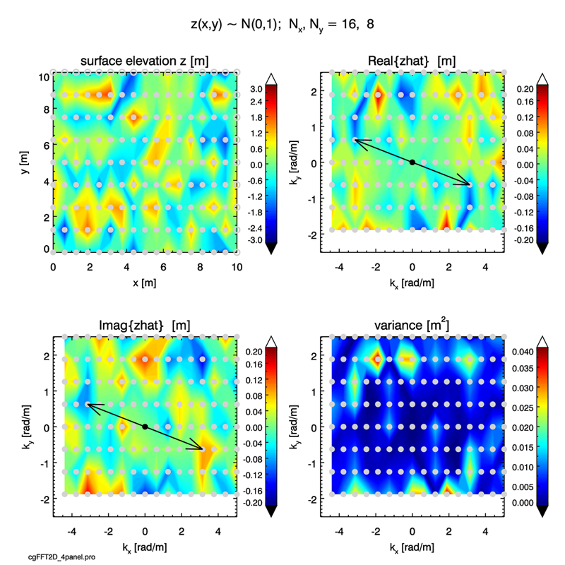
The Fourier amplitudes are obtained from the 2-D DFT of :
The usual warning on FFT frequency order applies here. The 2-D FFT gives back the amplitudes with the array elements corresponding the the FFT frequency order of Eq. (15) of the Fourier Transforms page. Before plotting, the array elements must be shifted into the math frequency order in both the and array directions using the appropriate shift function for the computer language used in the plotting. For the IDL routine used to generate Fig. 1, the 2-D circular shift is given by the IDL command
where zhat is the complex 2-D array returned by the FFT routine, and realzhatplot is the 2-D array plotted in the upper right panel of Fig. 1.
The upper right panel of Fig. 1 plots the real part of , and the lower left panel plots the imaginary part. The Nyquist frequency lies along the right side of the contour plot. The Nyquist frequency lies along the top of the contour plot. The white space at the left and bottom highlights that there are no negative Nyquist frequencies. In each amplitude plot a particular pair of values is indicated by the black arrows; the frequency is shown by a black dot. Note that in the plot of the real part, , whereas in the plot of the imaginary part, . The contouring is rather low quality for so few points, but it is easy to see in the digital output that when the is the Nyquist frequency (the points along the right column of points in the plot), the symmetries are given by and . A corresponding relation holds for when (the points along the top row of the plot). The point at the upper right of the plot corresponds to both and being at their respective Nyquist frequencies. As always, the array elements at the Nyquist frequencies must be treated as special cases when writing computer programs. These symmetries show that the 2-D amplitudes are Hermitian: . The discrete 2-D variance spectrum is contoured in the lower right panel of the figure. Note the symmetry.
For this example, the standard check on the 2-D discrete Parseval’s relation, Eq. (16) on page Fourier Transforms, gives
In all of these plots, it should be remembered that the discrete values are known only at the locations of the silver dots. The contouring routine simply interpolates between these points to create a visually appealing figure. The continuous color in the plots does not imply that the values are continuous and known in between the discrete points.
Example: A Sea Surface of Crossing Sinusoids
For a second example, let us define a surface from a pair of crossing sinusoids as follows:
| (2) |
where as usual and where
- is the amplitude of the first wave
- is the number of wave lengths in the x direction in for the first wave
- is the frequency of the first wave
- is the number of wave lengths in the y direction in for the first wave
- is the frequency of the first wave
- is the phase of the first wave; 0 gives a cosine wave
- is the amplitude of the second wave
- is the number of wave lengths in the x direction in for the second wave
- is the frequency of the second wave
- is the number of wave lengths in the y direction in for the second wave
- is the frequency of the first wave
- is the phase of the second wave; gives a sine wave
The wavelength of the first wave is , and that of the second wave is . The direction of propagation of the first wave relative to the axis is
and the direction of propagation of the second wave relative to the axis is
The upper left panel of Fig. 2 shows this surface elevation pattern when Eq. (2) is sampled with . The dominant red-blue pattern shows the first wave oriented with the direction of propagation along either the direction at or the direction at . We cannot of course determine the actual direction or of propagation from sea surface elevations at a single time. The dominant wave pattern is modulated by the second wave, which has one half the amplitude of the first wave.
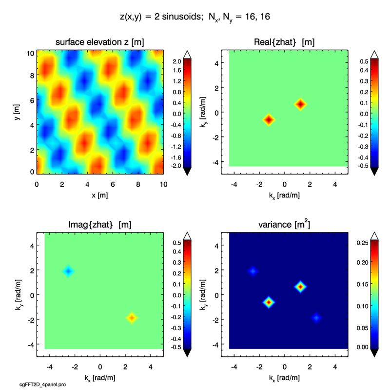
The choice above of in Eq. (2) makes the dominate wave a cosine in our coordinate system, and makes the second wave a sine. As we saw in the 1-D examples, variance associated with cosine waves appears in the real part of the Fourier amplitudes, and the variance in sine waves appears in the imaginary parts. We see this again here for the first (cosine) and second (sine) waves of the surface. Since each wave pattern has only one frequency, there is only one pair of points at in the plot of the real part, and one pair at in the plot of the imaginary part. The amplitudes at all other frequencies are zero. The symmetries of these points again show the Hermitian nature of the amplitudes.
The lower right panel shows the two-sided variance function for this surface. Note that the first wave has four times the variance of the second wave because the amplitude of the first wave is twice that of the second wave. . Note also that you can look at a 2-D variance spectrum and see how much energy is propagating in a given direction.
For this simple example involving just four frequencies it is easy (from the digital output) to hand check that the right-hand side of the 2D discrete Parseval’s relation, Eq. (18) of the Fourier Transforms page, is
This value agrees exactly with the corresponding sums of the surface elevations, , and variance values, .
 See comments posted for this page and leave your own.