Page updated:
March 13, 2021
Author: Curtis Mobley
View PDF
Chlorophyll Fluorescence
This page tailors the general fluorescence theory seen on the Theory of Fluorescence and Phosphorescence page to the case of fluorescence by chlorophyll in living phytoplankton. The goal is to develop the quantities needed for prediction of chlorophyll fluorescence contributions to oceanic light fields using a radiative transfer model like HydroLight. For convenience of reference, it is recalled from the previous page that the quantities needed are
- the chlorophyll fluorescence scattering coefficient , with units of ,
- the chlorophyll fluorescence wavelength redistribution function , with units of , and
- the chlorophyll fluorescence scattering phase function , with units of .
These quantities are then combined to create the volume inelastic scattering function for chlorophyll fluorescence,
| (1) |
The subscript C indicates chlorophyll.
The Chlorophyll Fluorescence Scattering Coefficient
For chlorophyll fluorescence, the inelastic “scattering” coefficient in the formalism of treating the fluorescence as inelastic scattering is just the absorption coefficient for chlorophyll. In other words, what matters is how much energy is absorbed by chlorophyll at the excitation wavelength , which is then available for possible re-emission at a longer wavelength . Note that it is only energy absorbed by the chlorophyll molecule that matters for chlorophyll fluorescence. Energy absorbed by other pigments may (or may not) fluoresce, but that is not chlorophyll fluorescence. Thus the needed chlorophyll scattering coefficient is commonly modeled as
where is the chlorophyll profile in and is the chlorophyll-specific absorption spectrum in units of . Examples of these spectra are seen on the Phytoplankton page. (The elastic scattering coefficient for chlorophyll-bearing phytoplankton is often modeled as a power law, as described on the New Case I IOPs.)
The Chlorophyll Fluorescence Wavelength Redistribution Function
Figure 1 shows a typical chlorophyll fluorescence emission spectrum.
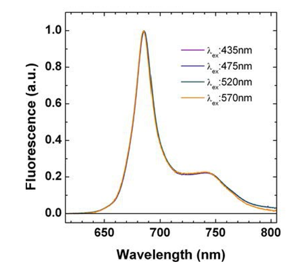
Other than the general shape, the important feature of this emission spectrum is that it is independent of the excitation wavelength. The chlorophyll absorption spectrum peaks in the blue and is a minimum in the green, so a 435 nm photon is much more likely to be absorbed by a chlorophyll molecule than is a 570 nm photon. However, either photon, if absorbed, leads to the same fluorsecence. Wavelengths in the range of 370 to 690 nm can, if absorbed, can lead to fluorescence. Given these observations, it is customary (e.g., Gordon (1979)) to factor the chlorophyll into a product of functions:
| (2) |
where
- is the quantum efficiency for chlorophyll fluorescence,
- is a nondimensional function that specifies the interval over which light is able to excite chlorophyll fluorescence, and
- is the chlorophyll fluorescence wavelength emission function, with units of .
The following sections describe how each of these terms can be modeled.
The quantum efficiency of chlorophyll fluorescence
The first factor on the right-hand side of Eq. (2), the quantum efficiency , is just a number, but it is the most difficult to model. This is because its value depends on the type and physiological state of the phytoplankton, and the physiological state is affected by the available light and nutrients, the temperature, and other factors.
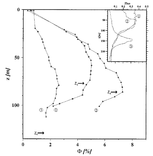
Figure 2 shows three depth profiles of determined as described in Maritorena et al. (2000). The locations were in oligotrophic areas of the equatorial Pacific where the chlorophyll values were between 0.035 and . The inset shows the fluorescence signal, which is proportional to the chlorophyll concentration and thus shows the shape of the profiles. The arrows labeled are the depths of the euphotic zone, which was defined as the depth where the irradiance has decreased to 1% of its surface value. The irradiance decreases approximately exponentially with depth, so the ordinate axis roughly corresponds to a log-scale plot of irradiance level. In the high-irradiance, near-surface region, the quantum efficiency is between 0.005 and 0.01. However, in the lower-irradiance regions below 50 m depth, is as large as 0.07. Very similar profiles can be seen in Fig. 8 of Morrison (2003).
Several models have been developed to predict as a function of the variables that affect it. Understanding these models requires a cellular-level understanding of the processes involved in photosynthesis, which is far beyond the level of this page. See, for example, Kirk (1994) for a general discussion of photosynthesis and Kiefer and Reynolds (1992) for discussion of the factors determining . In addition to PAR, these models depend on quantities such as the fraction of open photosystem II (PSII) reaction centers. An example model is that of Morrison (2003) (his Eq. 18), which has the form
| (3) |
where
- is the fraction of PSII reaction centers that are unaffected by nonphotochemical quenching
- is related to nonphotochemical quenching and ranges between 0 (maximum quenching) and 1 (minimal quenching)
- is the ambient scalar irradiance PAR in units of
- is the saturation PAR value for energy dependent nonphotochemical quenching
- and
- is the saturation PAR value for photosynthesis
- is the fraction of open PSII reaction centers
Quenching refers to any process that reduces the amount of fluorescence. These processes include the use of the absorbed energy for the chemical processes of photosynthesis (photochemical quenching) and the transfer of energy into heat (nonphotochemical quenching). Nonphotochemical quenching is common in phytoplankton as a way to protect themselves from the harmful effects of high irradiance levels. Quenching of whatever type reduces the energy available for re-emission as fluorescence and therefore reduces the quantum efficiency of fluorescence (with corresponding increases in the quantum efficiency of photosynthesis or of heating).
Figure 3 shows three curves for as a function of the ambient PAR , for values of and 1.0, which include the range of observed values seen in Fig. 8 of Morrison (2003). Note the similarity to the profiles seen in Fig. 2: values of less than 0.01 at high PAR values (i.e., near the surface), a maximum of around 0.06 at medium PAR values, and then decreasing for very low PAR values.
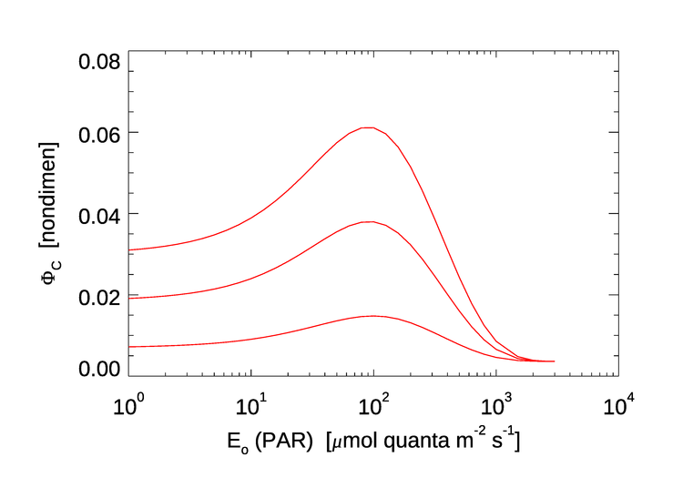
A more sophisticated model, including the effects of temperature and the surface chlorophyll concentration, is developed in Ostrovska (2012). That model gives curves qualitatively similar to those in Fig. 3, but with a maximum values up to 0.1 for some values of the temperature and surface chlorophyll concentration.
Thus measurements of (e.g., Fig. 2) and recent models (e.g., Eq. (3)) are in reasonable agreement. However, a model for in terms of PAR cannot be used in a radiative transfer model like HydroLight for the simple reason that the purpose of HydroLight is to predict the radiance and derived quantities, including PAR, by solving the radiative transfer equation (RTE), so the PAR values needed in Eq. 3 and similar models are not known until after the RTE has been solved. At best, HydroLight could be run once to compute the PAR profile, and then run again with that PAR profile used in Eq. (3) to compute the chlorophyll fluorescence contribution.
For this reason, the value of to be used in a HydroLight simulation is left as a user input to be chosen at run time. The default value in the current version 6 is . This is a mid-range value for moderate-irradiance, upper-ocean conditions, although Falkowski et al. (2017) report an average value of in surface waters for 200,000 profiles taken in a wide variety of locations.
The chlorophyll excitation function
As previously noted, wavelengths in the range of 370 to 690 nm, if absorbed, are equally likely to excite chlorophyll fluorescence. Therefore, is modeled by
The chlorphyll emission function
The emission function is commonly (e.g., Gordon (1979)) approximated as a Gaussian:
where
is the wavelength of maximum emission, and
is the standard deviation of the Gaussian; 10.6 nm corresponds to a full width at half maxmimum of , as seen in the equivalent second form of the function.
It should be noted that this , when used in the defined in Eq. (2) and integrated over as in Eq. (4) of the preceding theory page,
| (5) |
gives the quantum efficiency as required.
Figure 1 shows that this Gaussian captures only the main peak of the emission function. A better model for is a weighted sum of two Gaussians, one centered at 685 with a FWHM of 25 nm and one centered at 730 or 740 with a FWHM of 50 nm:
| (6) |
where and are the weights of the Gaussians at these wavelengths. These weights correspond to the fractions of the total quantum efficiency contributed by each Gaussian. Setting gives the peak height of the second Gaussian as 0.2 of the first, consistent with Fig. 1. Using (6) in (2) and (5) then again recovers .
The exact shape of the fluorescence emission seen in Fig. 1 and the corresponding best-fit parameters—heights and widths of the Gaussians and their center wavelengths—do vary somewhat with plankton species, pigment content and ratios, photoadaptation, nutrient conditions, stage of growth. and other parameters. This is, after all, why fluorescence gives information about the physiological state of phytoplankton.
The chlorophyll fluorescence phase function
As previously noted, fluorescence emission is isotropic. Therefore the phase function is simply
The models seen above give everything needed to construct the volume inelastic scattering function of Eq. (1) for chlorophyll fluoresecence, , which is then ready for use in the radiative transfer equation as seen in Eq. (2) of the theory page.
Examples of Chlorophyll Fluorescence Effects
The HydroLight radiative transfer model has options to include or omit the inelastic scattering processes of Raman scatter by water and fluorescence by chlorophyll and CDOM. This section uses HydroLight to illustrate the effects of various chlorophyll fluorescence input parameters.
To see the effect of the shape of the chlorophyll emission function, a series of four HydroLight runs was done with the following inputs:
- A chlorophyll concentration of for Case 1 water (using the New Case 1 IOP model in HydroLight); the water was homogeneous and infinitely deep
- A chlorophyll quantum efficiency of
- A chlorophyll emission function given by either Eq. (4) or (6)
- Sun at a zenith angle of 30 deg in a clear sky, wind speed of
- The run was from 400 to 750 nm by 5 nm
- Output was saved at 5 m intervals from 0 to 50 m
- Four sets of inelastic effects were simulated: (1) no inelastic effects at all, (2) Raman scatter only, (3) Raman scatter plus chlorophyll fluorescence with a single Gaussian emission function, and (4) Raman scatter plus chlorophyll fluorescence with a double Gaussian emission function
Figure 4 shows the the two Gaussian chlorophyll emission functions of Eqs. (4) and (6) (upper left panel); the resulting remote-sensing reflectance in the region of the chlorophyll emission (upper right panel); and the depth profiles of downwelling plane irradiance at 710 nm, (lower left); and at 730 nm, (lower right).
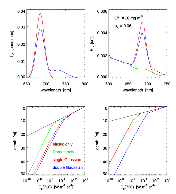
Some of the features to note in Fig. 4 are as follows:
- The peak values near 685 nm are larger for the single Gaussian than for the double Gaussian. This is because both emission functions, when integrated as in Eq. (5), correspond to the same quantum efficiency . Thus, as seen in the upper left panel, the 685 peak of the double Gaussian is lower than for the single Gaussian because part of the energy is going into the second Gaussian centered at 730 nm.
- There is no fluorescence contribution to for the single Gaussian beyond about 720 nm, but the double Gaussian gives a noticeable increase in even beyond 750 nm. This corresponds to the magnitudes of the two emission functions. However, magnitude of is quite small in the near infrared relative to the peak emission values and at shorter wavelengths (not shown) even for the high chlorophyll value of and the high efficiency of used here because of the high absorption by water itself beyond 700 nm; water absorption at 720 nm is and rises to at 750 nm.
- The profiles are similar down to about 5 m. For shallower depths, solar radiance at 710 nm penetrates the water column well enough to dominate the value of . Inelastic scatter contributions to the near-surface light field are minimal at 710 nm for these IOPs.
- Below about 10 m, the simulation without any inelastic scattering is greatly different from the curves with Raman or Raman plus fluorescence. Essentially the only light at 710 nm at depths below about 15 m comes from light at blue and green wavelengths, which do penetrate to depths below 15 m, that is inelastically scattered into 710 nm. As expected from the shapes of the emission functions, the double Gaussian “injects” more light into 710 nm than does the single Gaussian.
- At 730 nm, the Raman only and Raman plus single Gaussian emission are essentially identical because the single Gaussian is almost zero at 730. However, the double Gaussian emission function still adds a significant amount of light into the deep water column.
In summary, for wavelengths greater than about 700 nm there is a significant fractional difference in and in the irradiances at depth for the two chlorophyll emission functions. However, these differences are likely to be unimportant for practical oceanographic problems. It is hard to imagine applications where accurate predictions of irradiances are required in the near infrared at large depths.
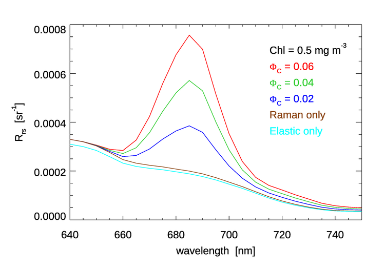
Figure 5 shows HydroLight simulations of in the chlorophyll fluorescence emission region for a value of , typical of open-ocean waters, and for three values of the quantum efficiency. The emission function is the double Gaussian. Other run inputs were the same as for Fig. 4. These curves include both Raman scatter and chlorophyll fluorescence. Curves for Raman only, and for elastic scatter only are also shown. Relative to the baseline of Raman only, the chlorophyll fluorescence curves are in direction proportion to the quantum efficiency values, all else being the same, as should be expected.
On the other hand, the height of the “Raman corrected” peak of the , double-Gaussian curve of the upper right panel of Fig. 4 is only about 6 times the height of the corresponding curve in Fig. 5, even though the chlorophyll concentration is 20 times higher for Fig 4. This is because absorption and scattering do not depend linearly on the chlorophyll concentration. For an order-of-magnitude understanding of this, note that it is absorption that removes light that might otherwise contribute to . The new Case 1 IOP model used for these runs models phytoplankton absorption by a formula that depends on . In the 400-680 nm range relevant to the chlorophyll fluorescence, ranges from 0.6 to 0.8. For a difference in chlorophyll values of 20, , which is close to the differences in the heights of the emission peaks. Absorption by CDOM will further reduce the light available for fluorescence.
 See comments posted for this page and leave your own.