Page updated:
May 7, 2021
Author: Curtis Mobley
View PDF
Inverse Problems
The development of the radiative transfer equation and its solution techniques in the chapter on radiative transfer theory has been concerned with the forward or direct problem of radiative transfer theory. The rules of the game were simple: Given the inherent optical properties of the water and the physical properties of the boundaries, find the radiance distribution throughout and leaving the water. This problem has a unique solution, which means that a given set of IOPs and boundary conditions yields a unique radiance distribution. The only limits on the accuracy of computed radiances are the accuracy with which we specify the IOPs and the boundary conditions, and the amount of computer time we wish to devote to the numerical solutions. In this sense the direct problem of computing radiances can be regarded as solved.
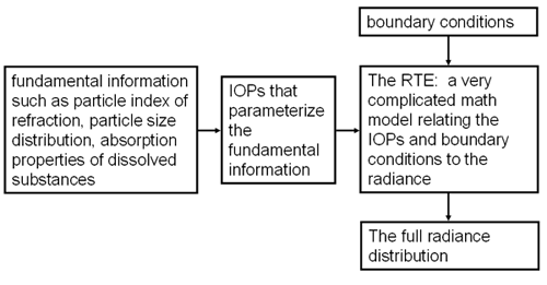
Figure 1 shows the conceptual process of solving the forward problem. In principle, we can start with the fundamental physical properties of the particles and dissolved substances in the ocean and derive the water IOPs from the physical properties (e.g., using Mie theory to compute the VSF from the particle properties and size distribution). In optical oceanography, we often being with direct measurements of the IOPs. We then apply suitable boundary conditions and solve the very complicated RTE to obtain the radiance distribution. Any other quantities of interest, such as irradiances or AOPs can then be computed from the radiances.
This page introduces the inverse problem of radiative transfer theory: given radiometric measurements of underwater or water-leaving light fields, determine the inherent optical properties of the water. This is very much an unsolved problem. Both conceptual and practical limits are encountered in inverse problems. Unfortunately, remote sensing is an inverse problem.
The first problem we encounter is uniqueness of the solution. Consider the following situation. A body of water with a particular set of IOPs and boundary conditions has an underwater radiance distribution . If the boundary conditions now change, perhaps because the sun moves, there will be a different radiance distribution within the water, even though the IOPs remain unchanged. Can we correctly recover the same set of IOPs from the two different light fields? Can we distinguish between because of a change in boundary conditions, as opposed to because of a change in IOPs? Because the same set of IOPs can yield different radiance distributions, as we just saw, we are led to ask if two different sets of IOPs and boundary conditions can lead to the same radiance distribution. In other words, is there even in principle a unique solution to the inverse problem stated above?
Another problem often encountered with inverse solutions is the stability of the solution, or its sensitivity to errors in the measured radiometric variables. In direct problems we often find that a small error (say 5%) in the IOPs or boundary conditions leads to a correspondingly small error in the computed radiance. With inverse problems we often find that small errors in the measured radiometric quantities lead to large errors, or even unphysical results, in the retrieved IOPs. Sensitivity of the inversion scheme to small errors in the input data often renders inversion algorithms useless in practice, even though they appear in principle to be quite elegant and satisfactory.
It can be shown that if the full radiance distribution is measured with perfect accuracy, there is in principle a unique inverse solution to the RTE to obtain the full set of IOPs. But from a practical standpoint, if we have to measure the entire radiance distribution throughout the water body with high accuracy to obtain the IOPs, we could measure the IOPs themselves just as easily. An inverse method is useful only when it saves us time, money, or effort. What is desired is a recovery of at least some of the IOPs from a limited set of imperfect radiometric measurements. We have seen one example of this in Gershun’s law, which allows us to recover the absorption coefficient from measured values of the plane and scalar irradiances, if there are no internal sources present.
In remote sensing, we have a very limited set of imperfect light field measurements, namely just the water leaving radiance or remote-sensing reflectance, from which we want to retrieve as much information as possible about the water body. Our input measurements fall far short of measuring the full radiance distribution, and the measurements we do have may contain substantial errors due to poor atmospheric correction or inaccurate radiometer calibration. Thus we expect a priori that we will not be able to recover a full set of water IOPs, and that what is recovered may contain large errors. Oceanic remote sensing is thus a very difficult inverse problem. The various inversion algorithms discussed on the following pages show the wide range of techniques developed over the years to address the inherent difficulties of inverting remote sensing measurements to obtain information about the ocean. Each of these techniques has its strengths and weaknesses, and each is imperfect, but each still has demonstrated great value to oceanographers.
Inversions are always based on an assumed model that relates what is known to what is desired. The inversion is then effected by using the known quantities as inputs to the model, whose output is an estimate of the desired quantities. In some cases the model is simple. For example, if historical data relating the chlorophyll concentration to the ratio of remote sensing reflectance at two wavelengths are used to find a best-fit function of the form , then the model is that function. Inserting a newly measured reflectance at and then gives an estimate of the chlorophyll concentration. The accuracy of that estimate will depend on the scatter in the original data, and on whether the water body being studied is similar to the one used to determine the function. In other cases the model is complicated. A neural network with may layers is a complex model in which it is often not obvious how a particular input is related to a particular output. The accuracy of a neural network inversion depends on how well the neural network represents nature and on the data used to train the network.
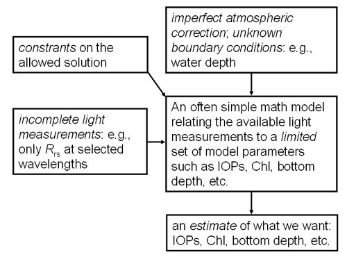
Because of the limited measurements available for remote sensing, inversion algorithms usually require constraints to limit the possible solutions obtained from a give remote sensing reflectance. Constraints can be “built in” for example as simplifications to the RTE. They can also be external, typically as additional required measurements (such as a measurement of the water leaving radiance or bottom depth at one point in an image). They can also be implicit constraints, such as a limitation of retrieved values to the range of values found in the data set used to pre-determine certain parameters in the inverse model.
Figure 2 summarizes the conceptual issues involved with inverting remotely sensed data to obtain estimates of oceanic properties.
Classification of inverse problems
There are many kinds of inverse problems. For example, there are medium characterization problems, for which the goal is to obtain information about the IOPs of the medium, which in our case is the water body with all of its constituents. This is the type of problem that we consider in this chapter. There are also hidden-object characterization problems, for which the goal is to detect or obtain information about an object imbedded within the medium, for example a submerged submarine. We shall not discuss this type of problem. Inverse problems may use optical measurements made in situ, as with the use of Gershun’s equation to obtain the absorption coefficient. Remote sensing uses measurements made outside the medium, typically from a satellite or aircraft.
Another type of inverse problem seeks to determine the properties of individual particles from light scattered by single particles. Such problems usually start with considerable knowledge about the particles (for example, the particles are spherical and have a known radius) and then seek to determine another specific bit of information (such as the particle index of refraction). The associated inversion algorithms usually assume that the detected light has been singly scattered. Even these highly constrained problems can be very difficult. We shall not discuss these “individual-particle” inverse problems. In the ocean, there is no escaping multiple scattering, which greatly complicates our problem, and we do not generally have the requisite a priori knowledge of the individual particle properties needed to constrain the inversion.
Solution techniques to inverse problems fall into two categories: explicit and implicit. Explicit solutions are formulas that give the desired IOPs as functions of measured radiometric quantities. A simple example is Gershun’s law when solved for the absorption in terms of the irradiances. Implicit solutions are obtained by solving a sequence of direct or forward problems. In crude form, we can imaging having a measured remote-sensing reflectance (or set of underwater radiance or irradiance measurements). We then solve direct problems to predict the reflectance for each of many different sets of IOPs. Each predicted reflectance is compared with the measured value. The IOPs associated with the predicted reflectance that most closely matches the measured reflectance are then taken to be the solution of the inverse problem. Such a plan of attack can be efficient if we have a rational way of changing the IOPs from one direct solution to the next, so that the sequence of direct solutions converges to the measured reflectance or radiance.
The follow pages show examples of both explicit and implicit inversions, with algorithms based on analytical simplifications of the RTE, on statistical fitting of functions to historical data sets, and on combinations of the two. Sometimes the underlying models and constraints will be obvious, and sometimes not. In any case, studying a remote-sensing algorithm in the general context of inverse models helps to ascertain what model underlies the algorithm, what its limitations and constraints are, and what is its expected domain of applicability.
 See comments posted for this page and leave your own.