Page updated:
March 14, 2021
Author: Curtis Mobley
View PDF
Error Estimation
This page shows how to estimate the errors in Monte Carlo simulations. General results from probability theory are illustrated with numerical examples.
To be specific, suppose that we need to estimate the fraction of power emitted by a light source that will be received by a detector. The answer of course depends on the water IOPs; the size, orientation, and location of the detector relative to the light source; the angular distribution of the emitted light; and perhaps on other things like boundary surfaces that can reflect or absorb light scattered onto the boundary. The numerical results to be shown below use the source and detector geometry shown in Fig. 1. The source emits a collimated bundle of rays toward a detector that is optical path lengths away and is optical path lengths in diameter. The water IOPs have and so that and one meter is one optical path length. The albedo of single scattering is . The scattering phase function is a Henyey-Greenstein phase function with a scattering-angle mean cosine of .
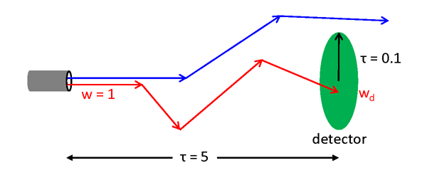
In the simulations, rays will be emitted from the source, each with an initial weight of . Most of those rays will miss the detector, as illustrated by the blue arrows in Fig. 1. However, some rays will hit the detector, as illustrated by the red arrows, at which time their current weight will be tallied to the accumulating total weight received by the detector. After all rays have been traced, the the Monte Carlo estimate of the fraction of emitted power received by the detector is simply .
If we do only one simulation tracing, say, ray bundles, then the resulting estimate of is all we have. In particular, we have no estimate of the statistical error in the estimated .
Probability Theory
To develop a quantitative error estimate for the result of a Monte Carlo simulation, we begin with a review of some results from basic probability theory. Recalling the notation introduced on the Monte Carlo Introduction page, let be the probability density function (pdf) for random variable . Capital represents the random variable, e.g. the ray bundle weight received by the detector, and lower case represents a specific value of , e.g., . In the present example, is the pdf that a ray strikes the detector with a weight . rays that miss the detector do not contribute to accumulating weight or power received by the detector and do not enter into the calculations below; they are simply wasted computer time. Note that we have no idea what mathematical form has: it results from a complicated sequence of randomly determined ray path lengths and scattering angles.
For any continuous pdf the expected or mean value of is defined as
| (1) |
where denotes expected value and the integral is over all values for which is defined. If the random variable is discrete, the integral is replaced by a sum over all allowed values of . Similarly, the variance of is defined as
Note that if is a constant, then
Greek letters and are used to denote the true or population mean and variance of a pdf.
Suppose that ray bundles actually reach the detector. The total weight received by the detector is then given by the sum of these randomly determined weights:
where is the weight of ray bundle when it reached the detector.
Each of the ray bundles emitted by the source and traced to completion is independent of the others. In particular, a different sequence of random numbers is used to determine the path lengths and scattering angles for each emitted bundle. Moreover, the underlying pdfs for ray path length and scattering angles (i.e., the IOPs) are the same for each bundle. The random variables are then said to be independent and identically distributed (iid), and is said to be a random sample of size of random variable .
The linearity of the expectation (i.e., the integral of a sum is the sum of the integrals) means that for iid random variables such as ,
| (2) |
In the Monte Carlo simulation, the sample mean, i.e. the estimate of the average detected weight obtained by from the detected ray bundles is
Equation (2) now gives two extremely important results. First,
| (3) |
That is, the expectation of the sample mean is equal to the true mean . The sample mean is then said to be an unbiased estimator of the true mean of the pdf. Second,
| (4) |
Thus, the variance of the sample mean goes to zero as , that is, as more and more ray bundles are detected. In other words, the Monte Carlo estimate of the average power received by the detector is guaranteed to give a result that can be made arbitrarily close to the correct result if enough rays are detected. This result is known as the law of large numbers. Again, you can emit and trace all the rays you want, but if they don’t hit the detector, they don’t count.
It is often convenient to think in terms of the standard deviation, e.g., when plotting data and showing the spread of values. The standard deviation of the error in is
| (5) |
The dependence of the standard deviation of the estimate on is a very general and important result. However, this “approach to the correct value” is very slow. If we want to reduce the standard deviation of the error in the estimated average power received by the detector by a factor of 10, we must detect 100 times as many rays. That can be computationally very expensive.
It is to be emphasized that result (4) that the variance of a sample mean equals the true variance divided by the sample size holds for any situation for which the individual samples are independent and identically distributed random variables.
Note, of course, that if we knew the pdf for the received power, , then we could simply evaluate Eq. (1) to get the desired true mean , and no Monte Carlo simulation would be required.
Finally, it must be remembered that the discussion here assumes that ”all else is the same” when considering the number of detected rays. For example, we emit and trace more rays without changing the physics of the simulation. The page on importance sampling presents ways to increase the number of detected rays and thereby reduce the variance, but with a change in the physics that sometimes may invalidate the simple dependence.
Numerical Examples
Numerical simulations were performed for the geometry and conditions described for Fig. 1. For these simulations, tracing type 1 of the previous page was used. That is, ray bundles were traced until they either hit the target (still with weight ) or were absorbed. For a given number of emitted ray bundles, various numbers of independent runs were done. That is, rays were traced and the number of detected ray bundles and their weights were tallied for each run. The fraction of emitted power received by the detector was then computed by the total detected weight for the run divided by . Then another run was made with everything the same except that a different sequence of random numbers was used (i.e., each run was started with a different seed for the random number generator used to determine path lengths and scattering angles).
The first set of simulations used emitted ray bundles for each run, with , and 10,000 runs being made. Figure 2 shows the distributions of the sample means and other information for these four sets of run numbers. The upper left panel of the figure is for only runs, or trials, or simulations. In this panel, the histogram shows that one run, or 0.1 of the total number of runs, gave an estimated fraction between 0.0088 and 0.0090 of the emitted power; two runs, or 0.2 of the total, gave a fraction between 0.0104 and 0.0106, and so on. As the number of runs increases, the estimates of the fraction of power received range from slightly less than 0.008 to slightly more than 0.014, with most estimates centering somewhere near 0.0108.
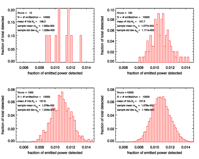
As the number of runs increases, something very remarkable happens: the distribution of the fraction of the emitted power appears to be approaching a Gaussian or normal shape, even though the underlying pdf is certainly not Gaussian. This distribution can be thought of as the distribution of errors in the estimated mean of the distribution, or the distribution of , where is the unknown true mean of the distribution . This approach to a Gaussian distribution is a consequence of the central limit theorem. The central limit theorem states that the sum of a large number of independently distributed random variables with finite means and variances is approximately normally distributed regardless of what the distribution of the random variable itself may be. This is one of the most profound results in probability theory. Indeed, it explains why so many natural phenomena tend to have a Gaussian shape. Phenomena as disparate as average student exam scores, noise in electrical circuits, daily water usage in a city, or the fraction of people who develop cancer can all result from sums of many individual contributions. Such sums then tend toward a Gaussian distribution as the number of individual contributions increases. The theorem was first proved for a specific pdf in 1733, but it was not proven to hold for all pdfs (having finite means and variances) until the early 1900’s. (By the way, in spite of what you see in the tabloid press, there is nothing in probability theory called “the law of averages.” The central limit theorem is maybe the closest thing to the often involked buy mythical “law of averages.”)
Figure 3 shows the corresponding results for series of , and 10,000 runs being made, but with each run now having emitted rays. Now the spread in the estimated values is much less, from slightly less than 0.010 to about 0.012, again centering somewhere around 0.0108. Again, we see the approach to a Gaussian shape as more and more runs are made, but the Gaussian has a narrower width, i.e. less variance about the mean. The standard deviation of the sample estimates of the mean is usually called the “standard error of the mean.”
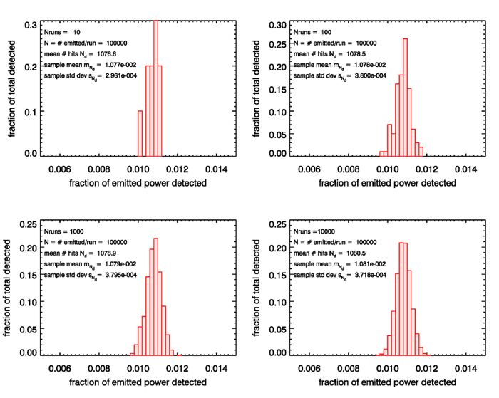
The lower right panel of Fig. 2 shows that the sample standard deviation for the case of 10,000 runs each with 10,000 emitted rays is and the average number of detected rays is . The corresponding panel of Fig. 3 shows and . The ratio of these sample standard deviations is
The corresponding ratio of values is
This nicely illustrates the dependence of the sample standard deviation, or the standard error of the mean, on the square root of the number of ray bundles detected, just as predicted by Eq. (5).
Error Estimation
In the present example of the fraction of emitted power received by a detector, the central limit theorem guarantees that the errors in the fraction of received power computed by many Monte Carlo runs approaches a Gaussian. We can thus use all of the results for Gaussian, or normal, probability distributions to estimate the errors in the Monte Carlo results.
It is often desirable to know the probability that the computed sample mean is within some prechosen amount, say 1 standard deviation, of the (unknown) true mean . Conversely, we may want to compute the error range so that the sample mean is within that error range of the true mean with some prechosen probability. Such questions can be answered starting with the statement
This equation states that the probability is that the sample mean is within a range of the true mean ; is a fraction of the sample standard deviation . In other words, the probability is that . The central limit theorem guarantees that, if the sample size is large enough, the deviation of the sample mean from the true mean, , is approximately normally distributed:
| (6) |
Assuming that we have enough samples to get a good approximation to the normal distribution, the probability that is greater than by an amount is then
Letting gives
| (7) |
The integral in the last equation cannot be performed analytically, but it is tabulated in probability texts, and software packages such as MATLAB and IDL have routines to compute it. In to also common to find tables and subroutines for
Note that .
Let us now apply Eq. (7) to various examples. We first compute the probability that the sample mean is within one standard deviation of the true mean. Letting , we compute the probability that lies in the “right-hand tail” of the normal distribution beyond . This is the area shaded in red in Fig. 4.
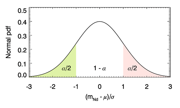
This probability is
, so . The Gaussian distribution is symmetric about the mean, so that lies in the left-hand (green-shaded) tail of the distribution also equals 0.1587. Thus the probability that does not lie in either tail of the distribution, i.e. that is .
For the simulations of Fig. 2, the lower right panel shows values of and . Thus there is a roughly 68% chance that the true fraction of received power is within the range . For the corresponding run of Fig. 3, which traced ten times as many ray bundles, the corresponding numbers are . Thus, in the last set of simulations, we are 68% certain that the sample mean is within about of the true mean.
Suppose we need the probability that we are within, say, 5% of the correct value. For the lower right simulation of Fig. 3, 0.05 of 0.01081 is about 0.00054. From we get . , so the probability of being within 5% is . If being 85% confident that the Monte Carlo estimate of the mean is within 5% of the true value is adequate for your application, then you are done. If you need to be 95% confident that you are within 5% of correct, then you need to continue tracing rays until you get enough rays on the target to reduce the sample variance to a value small enough to achieve the desired 95% confidence.
As a final example, we might ask how big is the error so that we can say that we are within that range with 90% certainly. We now set , and solve
Again, the inverse of is also tabulated. This equation gives . From the last panel of Fig. 3 we then get , so that with 90% confidence.
As a final caveat to this section, keep in mind that the central limit theorem says that the error becomes Gaussian as the number of samples, in the present examples, becomes very large. How large is large enough depends on the particular problem and the user’s accuracy requirement. In the present examples, 10,000 runs each with 10,000 or more emitted rays, resulting in 100 or more detected rays for each run, gives distributions that visually appear close to Gaussian (the lower right panels of the preceding two figures). There are various ways to quantify how close a data distribution is to a Gaussian, but that is a topic for somewhere else. Just do a search on ”normality tests.”
 See comments posted for this page and leave your own.