Page updated:
March 6, 2021
Author: Curtis Mobley
View PDF
Polarization: Scattering Geometry
This page discusses the geometrical considerations underlying computations of the scattering of polarized light using Stokes vectors. [Note to the reader: This page uses bold face for vectors in 3D space. This shows up well on the web page for Latin letters, but not as well for Greek letters, so use your common sense. The “blackboard” font is used for Stokes vectors () and rotation () and Mueller () matrices.]
As is shown on the Polarization: Stokes Vectors page, the state of polarization of a light field is specified by the four-component Stokes vector, whose elements are related to the complex amplitudes of the electric field vector resolved into directions that are parallel () and perpendicular () to a conveniently chosen reference plane.
However, there are two versions of the Stokes vector seen in the literature, and these two versions have different units and refer to different physical quantities. The coherent Stokes vector describes a quasi-monochromatic plane wave propagating in one exact direction, and the vector components have units of power per unit area (i.e., irradiance) on a surface perpendicular to the direction of propagation. To be specific, the coherent Stokes vector can be defined as (e.g., Mishchenko et al. (2002))
| (1) |
Here is the electric permittivity of the medium (with units of or SI units of ), and is the magnetic permeability of the medium ( or ). Electric fields have units of or . Thus the elements of the coherent Stokes vector have units of or (i.e., irradiance). denotes complex conjugate, hence the components of the Stokes vector are real numbers.
The diffuse Stokes vector is defined as in Eq. (1) but describes light propagating in a small set of directions surrounding a particular direction and has units of power per unit area per unit solid angle (i.e., radiance). It is the diffuse Stokes vector that appears in The General Vector Radiative Transfer Equation. The differences in coherent and diffuse Stokes vectors are rigorously presented in Mishchenko (2008b).
Authors often omit the factor in Eq. (1) because they are interested only in relative values such as the degree of polarization, not in absolute magnitudes, but this omission is both confusing and physically incorrect. Units and magnitudes matter! The different units of coherent and diffuse Stokes vectors, and whether or not the factor is included in the definition of the Stokes vector, have subtle but very important consequences in how light propagation across a dielectric interface such as the air-water surface is formulated. The recent paper by Zhai et al. (2012) gives a definitive discussion of these matters.
Coordinate Systems
To describe the scattering of polarized light, we must first choose coordinate systems and show in detail how to resolve Stokes vectors in these coordinate systems as needed for scattering calculations.
Figure 1 shows the coordinate systems commonly used to resolve Stokes vectors as needed for geophysical scattering calculations. In oceanography, depth and direction are defined in a 3D Cartesian coordinate system with depth measured positive downward from 0 at the mean sea surface. Polar angle is defined from 0 in the (or downwelling direction) to in the (upwelling) direction. is chosen for convenience, e.g., pointing toward the sun or pointing in the downwind direction (in which case is the cross-wind direction. As shown in Mobley (2014), using a wind-centered coordinate system makes it easier to model a random sea surface with different along-wind and cross-wind slope statistics.) Azimuthal angle is measured counterclockwise from when looking in the direction. If the Sun is placed in the azimuthal direction at , unscattered rays from the Sun are then traveling in the direction at deg.
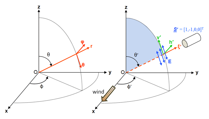
The unit vectors in the directions of increasing are
Let denote a unit vector pointing in the direction of light propagation, as given by angles . (In Fig. 1, .) The components of are given by
In radiative transfer theory, direction always refers to the direction of light propagation. Thus light traveling straight down is traveling in the or direction. To detect radiance in the direction, an instrument is pointed in the viewing direction , which is sometimes more convenient for plotting. A prime generally denotes an incident or unscattered direction, e.g, or . Unprimed variables denote final or scattered directions, e.g. or .
There is frequent need to resolve Stokes vectors in directions perpendicular and parallel to a given plane, which can be a meridian plane, a scattering plane in the water volume, or the plane of incident, reflected, and transmitted light for light incident onto an air-water or bottom surface. The following conventions define these unit vectors. Vector denotes a vector parallel to a plane, and denotes a vector perpendicular to a plane (“s” for senkrecht, German for perpendicular). The perpendicular vector is chosen to be in the direction given by the vector cross product of the incident direction crossed with the final direction. The parallel vector is then defined as the direction of propagation cross the perpendicular direction. Thus the perpendicular cross parallel directions give the direction of light propagation: , where denotes the vector cross product.
For an incident direction and the associated Stokes vector specified in the incident meridian plane, the first vector is taken to be and the second is the direction of propagation. Thus as seen in the right panel of Fig. 1. In this case , and . Similarly, , and . Meridian planes are perpendicular to the mean sea surface. The vector as just defined is therefore parallel to the mean sea surface and therefore is often referred to as the “horizontal” direction; lies in a vertical plane and is correspondingly called the “vertical” direction. For a final direction and its Stokes vector in the final meridian plane, the first vector is the direction and the second is z. This vector cross product algorithm for specifying perpendicular and parallel directions will be convenient for sea surface reflectance and transmission calculations in which light can propagate from one tilted wave facet to another without reference to meridian planes, except for the incident and final directions when a photon enters or leaves the region of the sea surface.
The and components of a Stokes vector describe linear polarization with the plane of polarization specified relative to a particular coordinate system. The component is the total radiance, and describes circular polarization; these quantities do not depend on the coordinate system and are invariant under a rotation of the coordinate system. The blue arrows in Fig. 1 represent the plane of oscillation of the electric field vector parallel to the meridian plane, i.e. for vertical plane polarization. The components of as shown thus represent radiance of magnitude that is 100% vertically plane polarized.
Scattering Geometry
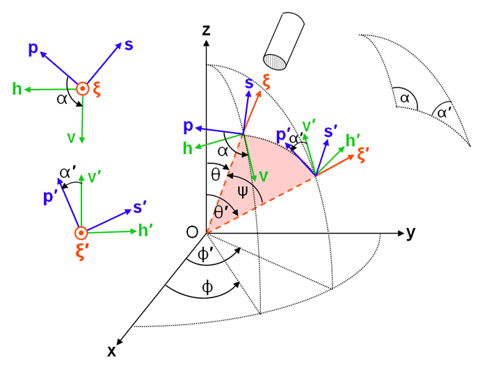
The elements of input and output Stokes vectors are defined relative to meridian planes, as described above. However, scattering from an incident direction to a final direction is defined in terms of the included scattering angle and the scattering plane, as illustrated in Fig. 2. Using Eqs. (5)-(8) to express the incident direction and scattered direction in terms of the incident and scattered polar and azimuthal angles gives the scattering angle :
Consider an incident beam of light propagating in direction as in Fig. 1. Direction is specified by polar and azimuthal directions . Primed variables denote unscattered or incident directions; unprimed variables denote scattered or final directions. The axis and the direction of light propagation define the incident meridian plane, part of which is shaded in blue in the right panel of Fig. 1. The (diffuse) Stokes vector for this beam of light is described with reference to “horizontal” and “vertical” directions, and respectively, which were defined above; the superscript T denotes transpose. Note that the horizontal unit vector is perpendicular to the meridian plane, and the vertical vector is parallel to the meridian plane.
To compute how an incident Stokes vector is scattered to a final vector , the horizontal and vertical components of in the incident meridian plane must first be transformed (“rotated”) into components parallel and perpendicular to the scattering plane. The coordinate system after rotation of and about the axis is labeled (parallel to the scattering plane) and (perpendicular to the scattering plane). Note that still gives the direction of propagation . As shown in Fig. 2, rotation angle takes into (and into ). In the present discussion, rotation angles are defined as positive for counterclockwise rotations when looking “into the beam,” e.g. in the direction. This is similar to rotations about the axis of Fig. 1 having positive angles for counterclockwise rotations when looking in the direction.
When computing single scattering with both and being expressed in their respective meridian planes, the rotation angles can be obtained from spherical trigonometry applied to the triangle defined by z, , and , which is shown in the inset in Fig. 2. Given , spherical trigonometry gives the rotation angles and as (e.g., Vol. 2, page 499 of van de Hulst (1980), or page 90 of Mishchenko et al. (2002))
| (10) |
or
| (11) |
and
| (12) |
or
| (13) |
for and for . If , then and are given by the negatives of these equations. The scattering angle is given by Eq. (9). The rotation and scattering angles depend only on the difference in azimuthal angles via . Special cases are required when , , or are zero. For , set since . For , set since . If , replace Eqs. (10) and (12) with Hu et al. (2001)
If , replace Eqs. (10) and (12) with
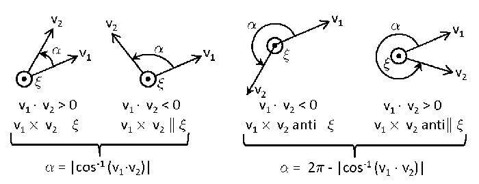
When doing calculations of multiple scattering between sea surface wave facets, a light ray can reflect from one wave facet to another several times before the incident ray finally leaves the surface region and needs to be rotated into the final meridian plane. In this case, it is more convenient to obtain the rotation angles from the perpendicular (or parallel) axes as determined for the incident ray direction onto a facet and the normal to the tilted wave facet. The details of these calculations are given in Mobley (2015) and will not be repeated here because they are not of general interest. However, it can be seen from Fig. 2 that the rotation angles can be obtained from and , where the dot denotes the vector dot or inner product. Figure 3 illustrates this for general initial and final vectors.
Once the incident Stokes vector is specified in the scattering plane, the scattering matrix is applied to obtain the final Stokes vector, which is then expressed in the s-p- scattering plane coordinate system defined for the final direction: . Finally, the parallel and perpendicular components of the final Stokes vector must be expressed as horizontal and vertical components in the final meridian plane as specified by the h-v- system. As illustrated in Fig. 2, this requires a counterclockwise rotation through an angle of , where is the “interior” angle of the spherical triangle illustrated in the figure. If represents a counterclockwise (positive) rotation through angle and represents scattering through scattering angle , then this scattering process is symbolically represented by
| (18) |
For the choice of a positive rotation being counterclockwise when looking into the beam, the Stokes vector rotation matrix is (e.g., Mishchenko et al. (2002)) page 25)
| (19) |
These rotation matrices have several obvious but important properties:
Equation (20) shows that rotating a coordinate system through an angle of , which turns s and p into -s and -p leaves the Stokes vector unchanged, consistent with the previous remark about directions -s, -p being equivalent to s, p as regards Stokes vectors. That is, Stokes vectors are referred to a plane, not to a particular direction in that plane.
It is noted for completeness that a rotation in 3D space by angle about an axis specified by unit vector is
| (25) |
for a counterclockwise rotation when looking in the direction. Although not needed for Stokes vector manipulations, this matrix can be used to check quantities determined by other means. For example, as seen in Fig. 2.
The choice of coordinate systems and rotation angles is not unique. Kattawar and Adams (1989), Kattawar (1994),Zhai et al. (2012), and Mishchenko et al. (2002)) all choose the reference plane to the be meridian plane. (These authors use somewhat different notation; our and are Kattawar’s and , respectively. Mishchenko et al. (2002)) (page 16) on the other hand use the spherical coordinate system unit vectors and for the vertical and horizontal axes.) Thus in the ocean setting they regard the “horizontal” direction (parallel to the mean sea surface) as being the “perpendicular” direction (relative to the meridian plane), and “vertical” to the mean sea surface as being the “parallel” direction. Note in Eq. (1) that if the parallel component of the electric field is zero, then the second element of the Stokes vector is proportional to , which is a negative number. A Stokes vector for light reflected from the sea surface with horizontal linear polarization is therefore proportional to , which they refer to as perpendicular polarization. Their choice of the reference plane means that the scattering (Mueller) matrix that transmits only horizontally polarized light has the form
| (26) |
However, Bohren and Huffman (1983)) and Hecht (1989) choose their “parallel” direction to be parallel to a horizontal direction, such as a laboratory bench top or the mean sea surface, and their vertical direction is perpendicular to the bench top or mean sea surface. Thus their Stokes vector for horizontal polarization (parallel to the mean sea surface) is and their Mueller matrix that transmits only horizontally polarized light has the form
The difference choices arise perhaps from the viewpoints of describing polarization in a convenient way for a laboratory experiment with reference to a table top, versus modeling light incident onto the sea surface with reference to meridian planes.
The forms of scattering matrices as commonly used to model scattering within the ocean and atmosphere are discussed on the VRTE for Mirror-symmetric Media page.
Similar confusion is found in the choice of rotation angles. Kattawar (and his students in their papers) and Bohren and Huffman (1983)) define a positive rotation as being clockwise when looking into the beam. Since a clockwise rotation through angle is the same as a counterclockwise rotation through , Kattawar’s rotation matrix is the transpose of the one in Eq. (19) (see Eq. 23). Thus Kattawar (e.g., in Eq. 10 of Kattawar and Adams (1989)) writes Eq. (18) as (again, with minor differences in notation; here is Kattawar’s , etc.). Others often write a rotation as rather than ; these are equivalent because by Eq. (19) shows that . Chandrasekhar (1960) also defines a positive rotation as being clockwise when looking into the beam. However, he uses a different definition for the Stokes vector for which only the fourth component is independent of coordinate system, so his rotation matrix is more complicated. Mishchenko defines a positive rotation as being clockwise when looking in the direction of propagation. This is equivalent to counterclockwise when looking into the beam as used here; thus his rotation matrix is the same as that in Eq. (19). van de Hulst (1980) also uses the same rotation convention as is used here. All of this is considered “well known,” so the details are often omitted in publications, with confusing apparent differences being the price of brevity. Fortunately, the only real requirement for Stokes vectors, coordinate systems, and rotations is consistency in usage once a choice has been made.
I’ll be the first to admit that this discussion of Stoke’s vector rotations is complicated and probably confusing. However, if you think it is bad reading about this business, just wait until you have to write a computer program to do these calculations.
 See comments posted for this page and leave your own.